{
"cells": [
{
"cell_type": "markdown",
"metadata": {
"execution": {}
},
"source": [
"[](https://colab.research.google.com/github/neuromatch/climate-course-content/blob/main/tutorials/W2D1_AnEnsembleofFutures/student/W2D1_Tutorial3.ipynb)  "
]
},
{
"cell_type": "markdown",
"metadata": {
"execution": {}
},
"source": [
"# Tutorial 3: Quantifying Uncertainty in Projections\n",
"\n",
"**Week 2, Day 1, An Ensemble of Futures**\n",
"\n",
"**Content creators:** Brodie Pearson, Julius Busecke, Tom Nicholas, Sam Ditkovsky\n",
"\n",
"**Content reviewers:** Mujeeb Abdulfatai, Nkongho Ayuketang Arreyndip, Jeffrey N. A. Aryee, Younkap Nina Duplex, Sloane Garelick, Paul Heubel, Zahra Khodakaramimaghsoud, Peter Ohue, Jenna Pearson, Abel Shibu, Derick Temfack, Peizhen Yang, Cheng Zhang, Chi Zhang, Ohad Zivan\n",
"\n",
"**Content editors:** Paul Heubel, Jenna Pearson, Ohad Zivan, Chi Zhang\n",
"\n",
"**Production editors:** Wesley Banfield, Paul Heubel, Jenna Pearson, Konstantine Tsafatinos, Chi Zhang, Ohad Zivan\n",
"\n",
"**Our 2024 Sponsors:** CMIP, NFDI4Earth"
]
},
{
"cell_type": "markdown",
"metadata": {
"execution": {}
},
"source": [
"# Tutorial Objectives\n",
"\n",
"*Estimated timing for tutorial:* 40 minutes\n",
"\n",
"In the previous tutorial, we constructed a *multi-model ensemble* using data from a diverse set of five CMIP6 models. We showed that the projections differ between models due to their distinct physics, numerics and discretizations. In this tutorial, we will calculate the uncertainty associated with future climate projections by utilizing this variability across CMIP6 models. We will establish a *likely* range of projections as defined by the IPCC. \n",
"\n",
"By the end of this tutorial, you will be able to \n",
"- Apply IPCC confidence levels to climate model data,\n",
"- Quantify the uncertainty associated with CMIP6/ScenarioMIP projections.\n"
]
},
{
"cell_type": "markdown",
"metadata": {
"execution": {}
},
"source": [
"# Setup\n",
"\n",
" \n",
"\n"
]
},
{
"cell_type": "code",
"execution_count": null,
"metadata": {
"execution": {},
"executionInfo": {
"elapsed": 21927,
"status": "ok",
"timestamp": 1683930403085,
"user": {
"displayName": "Brodie Pearson",
"userId": "05269028596972519847"
},
"user_tz": 420
},
"tags": [
"colab"
]
},
"outputs": [],
"source": [
"# installations ( uncomment and run this cell ONLY when using google colab or kaggle )\n",
"\n",
"# !pip install condacolab &> /dev/null\n",
"# import condacolab\n",
"# condacolab.install()\n",
"\n",
"# # Install all packages in one call (+ use mamba instead of conda), this must in one line or code will fail\n",
"# !mamba install \"xarray==2024.2.0\" xarray-datatree intake-esm gcsfs xmip aiohttp nc-time-axis cf_xarray xarrayutils &> /dev/null"
]
},
{
"cell_type": "code",
"execution_count": null,
"metadata": {
"execution": {},
"executionInfo": {
"elapsed": 3609,
"status": "ok",
"timestamp": 1683930517522,
"user": {
"displayName": "Brodie Pearson",
"userId": "05269028596972519847"
},
"user_tz": 420
},
"tags": []
},
"outputs": [],
"source": [
"# imports\n",
"import intake\n",
"import matplotlib.pyplot as plt\n",
"import xarray as xr\n",
"\n",
"from xmip.preprocessing import combined_preprocessing\n",
"from xmip.postprocessing import _parse_metric\n",
"from datatree import DataTree"
]
},
{
"cell_type": "markdown",
"metadata": {},
"source": [
"## Install and import feedback gadget\n"
]
},
{
"cell_type": "code",
"execution_count": null,
"metadata": {
"cellView": "form",
"execution": {},
"tags": [
"hide-input"
]
},
"outputs": [],
"source": [
"# @title Install and import feedback gadget\n",
"\n",
"!pip3 install vibecheck datatops --quiet\n",
"\n",
"from vibecheck import DatatopsContentReviewContainer\n",
"def content_review(notebook_section: str):\n",
" return DatatopsContentReviewContainer(\n",
" \"\", # No text prompt\n",
" notebook_section,\n",
" {\n",
" \"url\": \"https://pmyvdlilci.execute-api.us-east-1.amazonaws.com/klab\",\n",
" \"name\": \"comptools_4clim\",\n",
" \"user_key\": \"l5jpxuee\",\n",
" },\n",
" ).render()\n",
"\n",
"\n",
"feedback_prefix = \"W2D1_T3\""
]
},
{
"cell_type": "markdown",
"metadata": {},
"source": [
"## Figure settings\n"
]
},
{
"cell_type": "code",
"execution_count": null,
"metadata": {
"cellView": "form",
"execution": {},
"executionInfo": {
"elapsed": 738,
"status": "ok",
"timestamp": 1683930525181,
"user": {
"displayName": "Brodie Pearson",
"userId": "05269028596972519847"
},
"user_tz": 420
},
"tags": [
"hide-input"
]
},
"outputs": [],
"source": [
"# @title Figure settings\n",
"import ipywidgets as widgets # interactive display\n",
"\n",
"plt.style.use(\n",
" \"https://raw.githubusercontent.com/neuromatch/climate-course-content/main/cma.mplstyle\"\n",
")\n",
"\n",
"%matplotlib inline"
]
},
{
"cell_type": "markdown",
"metadata": {},
"source": [
"## Helper functions\n"
]
},
{
"cell_type": "code",
"execution_count": null,
"metadata": {
"cellView": "form",
"execution": {},
"executionInfo": {
"elapsed": 2,
"status": "ok",
"timestamp": 1683930525501,
"user": {
"displayName": "Brodie Pearson",
"userId": "05269028596972519847"
},
"user_tz": 420
},
"tags": [
"hide-input"
]
},
"outputs": [],
"source": [
"# @title Helper functions\n",
"\n",
"def readin_cmip6_to_datatree(facet_dict):\n",
" # open an intake catalog containing the Pangeo CMIP cloud data\n",
" col = intake.open_esm_datastore(\n",
" \"https://storage.googleapis.com/cmip6/pangeo-cmip6.json\"\n",
" )\n",
"\n",
" # from the full `col` object, create a subset using facet search\n",
" cat = col.search(\n",
" source_id=facet_dict['source_id'],\n",
" variable_id=facet_dict['variable_id'],\n",
" member_id=facet_dict['member_id'],\n",
" table_id=facet_dict['table_id'],\n",
" grid_label=facet_dict['grid_label'],\n",
" experiment_id=facet_dict['experiment_id'],\n",
" require_all_on=facet_dict['require_all_on'] # make sure that we only get models which have all of the above experiments\n",
" )\n",
"\n",
" # convert the sub-catalog into a datatree object, by opening each dataset into an xarray.Dataset (without loading the data)\n",
" kwargs = dict(\n",
" preprocess=combined_preprocessing, # apply xMIP fixes to each dataset\n",
" xarray_open_kwargs=dict(\n",
" use_cftime=True\n",
" ), # ensure all datasets use the same time index\n",
" storage_options={\n",
" \"token\": \"anon\"\n",
" }, # anonymous/public authentication to google cloud storage\n",
" )\n",
"\n",
" cat.esmcat.aggregation_control.groupby_attrs = [\"source_id\", \"experiment_id\"]\n",
" dt = cat.to_datatree(**kwargs)\n",
"\n",
" return dt\n",
"\n",
"\n",
"def global_mean(ds: xr.Dataset) -> xr.Dataset:\n",
" \"\"\"Global average, weighted by the cell area\"\"\"\n",
" return ds.weighted(ds.areacello.fillna(0)).mean([\"x\", \"y\"], keep_attrs=True)\n",
"\n",
"\n",
"# Calculate anomaly to reference period\n",
"def datatree_anomaly(dt):\n",
" dt_out = DataTree()\n",
" for model, subtree in dt.items():\n",
" ref = dt[model][\"historical\"].ds.sel(time=slice(\"1950\", \"1980\")).mean()\n",
" dt_out[model] = subtree - ref\n",
" return dt_out\n",
"\n",
"\n",
"def plot_historical_ssp126_combined(dt):\n",
" for model in dt.keys():\n",
" datasets = []\n",
" for experiment in [\"historical\", \"ssp126\"]:\n",
" datasets.append(dt[model][experiment].ds.tos)\n",
"\n",
" da_combined = xr.concat(datasets, dim=\"time\")"
]
},
{
"cell_type": "markdown",
"metadata": {},
"source": [
"## Video 1: Quantifying Uncertainty in Projections\n"
]
},
{
"cell_type": "code",
"execution_count": null,
"metadata": {
"cellView": "form",
"execution": {},
"tags": [
"remove-input"
]
},
"outputs": [],
"source": [
"# @title Video 1: Quantifying Uncertainty in Projections\n",
"\n",
"from ipywidgets import widgets\n",
"from IPython.display import YouTubeVideo\n",
"from IPython.display import IFrame\n",
"from IPython.display import display\n",
"\n",
"\n",
"class PlayVideo(IFrame):\n",
" def __init__(self, id, source, page=1, width=400, height=300, **kwargs):\n",
" self.id = id\n",
" if source == 'Bilibili':\n",
" src = f'https://player.bilibili.com/player.html?bvid={id}&page={page}'\n",
" elif source == 'Osf':\n",
" src = f'https://mfr.ca-1.osf.io/render?url=https://osf.io/download/{id}/?direct%26mode=render'\n",
" super(PlayVideo, self).__init__(src, width, height, **kwargs)\n",
"\n",
"\n",
"def display_videos(video_ids, W=400, H=300, fs=1):\n",
" tab_contents = []\n",
" for i, video_id in enumerate(video_ids):\n",
" out = widgets.Output()\n",
" with out:\n",
" if video_ids[i][0] == 'Youtube':\n",
" video = YouTubeVideo(id=video_ids[i][1], width=W,\n",
" height=H, fs=fs, rel=0)\n",
" print(f'Video available at https://youtube.com/watch?v={video.id}')\n",
" else:\n",
" video = PlayVideo(id=video_ids[i][1], source=video_ids[i][0], width=W,\n",
" height=H, fs=fs, autoplay=False)\n",
" if video_ids[i][0] == 'Bilibili':\n",
" print(f'Video available at https://www.bilibili.com/video/{video.id}')\n",
" elif video_ids[i][0] == 'Osf':\n",
" print(f'Video available at https://osf.io/{video.id}')\n",
" display(video)\n",
" tab_contents.append(out)\n",
" return tab_contents\n",
"\n",
"video_ids = [('Youtube', 'IdFRDwzKlsg'), ('Bilibili', 'BV1ocGDetEti')]\n",
"tab_contents = display_videos(video_ids, W=730, H=410)\n",
"tabs = widgets.Tab()\n",
"tabs.children = tab_contents\n",
"for i in range(len(tab_contents)):\n",
" tabs.set_title(i, video_ids[i][0])\n",
"display(tabs)"
]
},
{
"cell_type": "markdown",
"metadata": {},
"source": [
"## Submit your feedback\n"
]
},
{
"cell_type": "code",
"execution_count": null,
"metadata": {
"cellView": "form",
"execution": {},
"tags": [
"hide-input"
]
},
"outputs": [],
"source": [
"# @title Submit your feedback\n",
"content_review(f\"{feedback_prefix}_Quantifying_Uncertainty_in_Projections_Video\")"
]
},
{
"cell_type": "markdown",
"metadata": {},
"source": [
"\n"
]
},
{
"cell_type": "code",
"execution_count": null,
"metadata": {
"cellView": "form",
"execution": {},
"pycharm": {
"name": "#%%\n"
},
"tags": [
"remove-input"
]
},
"outputs": [],
"source": [
"# @markdown\n",
"from ipywidgets import widgets\n",
"from IPython.display import IFrame\n",
"\n",
"link_id = \"dhx9a\"\n",
"\n",
"print(f\"If you want to download the slides: https://osf.io/download/{link_id}/\")\n",
"IFrame(src=f\"https://mfr.ca-1.osf.io/render?url=https://osf.io/{link_id}/?direct%26mode=render%26action=download%26mode=render\", width=854, height=480)"
]
},
{
"cell_type": "markdown",
"metadata": {},
"source": [
"## Submit your feedback\n"
]
},
{
"cell_type": "code",
"execution_count": null,
"metadata": {
"cellView": "form",
"execution": {},
"tags": [
"hide-input"
]
},
"outputs": [],
"source": [
"# @title Submit your feedback\n",
"content_review(f\"{feedback_prefix}_Quantifying_Uncertainty_in_Projections_Slides\")"
]
},
{
"cell_type": "markdown",
"metadata": {
"execution": {}
},
"source": [
"# Section 1: Loading CMIP6 Data from Various Models & Experiments"
]
},
{
"cell_type": "markdown",
"metadata": {
"execution": {}
},
"source": [
"First, lets load the datasets that we used in the previous tutorial, which spanned 5 models. We will use three CMIP6 experiments, adding the high-emissions (*SSP5-8.5*) future scenario to the *historical* and *SSP1-2.6* experiments used in the last tutorial.\n",
"\n"
]
},
{
"cell_type": "code",
"execution_count": null,
"metadata": {
"execution": {}
},
"outputs": [],
"source": [
"# selected CMIP6 models to explore\n",
"source_ids = [\"IPSL-CM6A-LR\", \"GFDL-ESM4\", \"ACCESS-CM2\", \"MPI-ESM1-2-LR\", \"TaiESM1\"]\n",
"\n",
"# dictionary of facets for query of surface temperature data\n",
"facet_dict = { \"source_id\":source_ids,\n",
" \"variable_id\":\"tos\",\n",
" \"member_id\":\"r1i1p1f1\",\n",
" \"table_id\":\"Omon\",\n",
" \"grid_label\":\"gn\",\n",
" \"experiment_id\":[\"historical\", \"ssp126\", \"ssp585\"],\n",
" \"require_all_on\":\"source_id\"\n",
" }\n",
"\n",
"# dictionary for query of cell area metric\n",
"facet_dict_area = { \"source_id\":source_ids,\n",
" \"variable_id\":\"areacello\",\n",
" \"member_id\":\"r1i1p1f1\",\n",
" \"table_id\":\"Ofx\",\n",
" \"grid_label\":\"gn\",\n",
" \"experiment_id\":\"historical\",\n",
" \"require_all_on\":\"source_id\"\n",
" }\n",
"# search for temperature and area data and return datatree objects\n",
"dt_ensemble = readin_cmip6_to_datatree(facet_dict)\n",
"dt_area = readin_cmip6_to_datatree(facet_dict_area)\n",
"\n",
"\n",
"# merge area metric into datatree object\n",
"dt_with_area = DataTree()\n",
"\n",
"for model, subtree in dt_ensemble.items():\n",
" metric = dt_area[model][\"historical\"].ds[\"areacello\"]\n",
" dt_with_area[model] = subtree.map_over_subtree(_parse_metric, metric)\n",
"\n",
"# average every dataset in the tree globally\n",
"dt_gm = dt_with_area.map_over_subtree(global_mean)\n",
"\n",
"for experiment in [\"historical\", \"ssp126\", \"ssp585\"]:\n",
" da = dt_gm[\"TaiESM1\"][experiment].ds.tos\n",
"\n",
"dt_gm_anomaly = datatree_anomaly(dt_gm)"
]
},
{
"cell_type": "markdown",
"metadata": {
"execution": {}
},
"source": [
"# Section 2: Quantifying Uncertainty in a CMIP6 Multi-model Ensemble\n",
"\n",
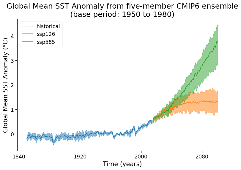
"Let's create a multi-model ensemble containing data from multiple CMIP6 models, which we can use to quantify our confidence in future projected sea surface temperature change under low- and high-emissions scenarios. \n",
"\n",
"**Your goal in this tutorial is to create a *likely* range of future projected conditions under both SSP 1-2.6 (low emissions) and SSP 5-8.5 (high emissions). The [IPCC uncertainty language](https://www.ipcc.ch/report/ar6/wg1/chapter/chapter-1/#h3-9-siblings) defines the *likely* range as the middle 66% of model results (ignoring the upper 17% and lower 17% of results)**"
]
},
{
"cell_type": "markdown",
"metadata": {
"execution": {}
},
"source": [
"### Coding Exercise 2.1\n",
"\n",
"Complete the following code to display multi-model ensemble data with IPCC uncertainty bands:\n",
"\n",
"1. Compute the multi-model mean temperature\n",
"2. Display the *likely* range of temperatures for the CMIP6 historical and projected data (include both *SSP1-2.6* and *SSP5-8.5*) via shaded areas with *da_upper* and *da_lower* being the boundaries of these shaded regions."
]
},
{
"cell_type": "code",
"execution_count": null,
"metadata": {
"execution": {}
},
"outputs": [],
"source": [
"#################################################\n",
"## TODO for students: Plot range of global mean SST anomaly for five-member ensemble##\n",
"# please remove the following line of code once you have completed the exercise:\n",
"raise NotImplementedError(\"Student exercise: Plot range of global mean SST anomaly for five-member ensemble\")\n",
"#################################################\n",
"\n",
"fig, ax = plt.subplots()\n",
"for experiment, color in zip([\"historical\", \"ssp126\", \"ssp585\"], [\"C0\", \"C1\", \"C2\"]):\n",
" datasets = []\n",
" for model in dt_gm_anomaly.keys():\n",
" # calculate annual mean\n",
" annual_sst = (\n",
" dt_gm_anomaly[model][experiment]\n",
" .ds.tos.coarsen(time=12)\n",
" .mean()\n",
" .assign_coords(source_id=model)\n",
" )\n",
" datasets.append(\n",
" annual_sst.sel(time=slice(None, \"2100\")).load()\n",
" ) # the french model has a long running member for ssp126\n",
" # concatenate all along source_id dimension\n",
" da = xr.concat(datasets, dim=\"source_id\", join=\"override\").squeeze()\n",
" # compute ensemble mean and draw time series\n",
" da.mean(...).plot(color=color, label=experiment, ax=ax)\n",
" # extract time coordinates\n",
" x = da.time.data\n",
" # Calculate the lower bound of the likely range\n",
" da_lower = da.squeeze().quantile(...)\n",
" # Calculate the upper bound of the likely range\n",
" da_upper = da.squeeze().quantile(...)\n",
" # shade via quantile boundaries\n",
" ax.fill_between(x, da_lower, da_upper, alpha=0.5, color=color)\n",
"\n",
"# aesthetics\n",
"ax.set_title(\n",
" \"Global Mean SST Anomaly from five-member CMIP6 ensemble\\n(base period: 1950 to 1980)\"\n",
")\n",
"ax.set_ylabel(\"Global Mean SST Anomaly (°C)\")\n",
"ax.set_xlabel(\"Time (years)\")\n",
"ax.legend()"
]
},
{
"cell_type": "markdown",
"metadata": {
"colab_type": "text",
"execution": {}
},
"source": [
"[*Click for solution*](https://github.com/neuromatch/climate-course-content/tree/main/tutorials/W2D1_AnEnsembleofFutures/solutions/W2D1_Tutorial3_Solution_3cfa2928.py)\n",
"\n",
"*Example output:*\n",
"\n",
"
"
]
},
{
"cell_type": "markdown",
"metadata": {
"execution": {}
},
"source": [
"# Tutorial 3: Quantifying Uncertainty in Projections\n",
"\n",
"**Week 2, Day 1, An Ensemble of Futures**\n",
"\n",
"**Content creators:** Brodie Pearson, Julius Busecke, Tom Nicholas, Sam Ditkovsky\n",
"\n",
"**Content reviewers:** Mujeeb Abdulfatai, Nkongho Ayuketang Arreyndip, Jeffrey N. A. Aryee, Younkap Nina Duplex, Sloane Garelick, Paul Heubel, Zahra Khodakaramimaghsoud, Peter Ohue, Jenna Pearson, Abel Shibu, Derick Temfack, Peizhen Yang, Cheng Zhang, Chi Zhang, Ohad Zivan\n",
"\n",
"**Content editors:** Paul Heubel, Jenna Pearson, Ohad Zivan, Chi Zhang\n",
"\n",
"**Production editors:** Wesley Banfield, Paul Heubel, Jenna Pearson, Konstantine Tsafatinos, Chi Zhang, Ohad Zivan\n",
"\n",
"**Our 2024 Sponsors:** CMIP, NFDI4Earth"
]
},
{
"cell_type": "markdown",
"metadata": {
"execution": {}
},
"source": [
"# Tutorial Objectives\n",
"\n",
"*Estimated timing for tutorial:* 40 minutes\n",
"\n",
"In the previous tutorial, we constructed a *multi-model ensemble* using data from a diverse set of five CMIP6 models. We showed that the projections differ between models due to their distinct physics, numerics and discretizations. In this tutorial, we will calculate the uncertainty associated with future climate projections by utilizing this variability across CMIP6 models. We will establish a *likely* range of projections as defined by the IPCC. \n",
"\n",
"By the end of this tutorial, you will be able to \n",
"- Apply IPCC confidence levels to climate model data,\n",
"- Quantify the uncertainty associated with CMIP6/ScenarioMIP projections.\n"
]
},
{
"cell_type": "markdown",
"metadata": {
"execution": {}
},
"source": [
"# Setup\n",
"\n",
" \n",
"\n"
]
},
{
"cell_type": "code",
"execution_count": null,
"metadata": {
"execution": {},
"executionInfo": {
"elapsed": 21927,
"status": "ok",
"timestamp": 1683930403085,
"user": {
"displayName": "Brodie Pearson",
"userId": "05269028596972519847"
},
"user_tz": 420
},
"tags": [
"colab"
]
},
"outputs": [],
"source": [
"# installations ( uncomment and run this cell ONLY when using google colab or kaggle )\n",
"\n",
"# !pip install condacolab &> /dev/null\n",
"# import condacolab\n",
"# condacolab.install()\n",
"\n",
"# # Install all packages in one call (+ use mamba instead of conda), this must in one line or code will fail\n",
"# !mamba install \"xarray==2024.2.0\" xarray-datatree intake-esm gcsfs xmip aiohttp nc-time-axis cf_xarray xarrayutils &> /dev/null"
]
},
{
"cell_type": "code",
"execution_count": null,
"metadata": {
"execution": {},
"executionInfo": {
"elapsed": 3609,
"status": "ok",
"timestamp": 1683930517522,
"user": {
"displayName": "Brodie Pearson",
"userId": "05269028596972519847"
},
"user_tz": 420
},
"tags": []
},
"outputs": [],
"source": [
"# imports\n",
"import intake\n",
"import matplotlib.pyplot as plt\n",
"import xarray as xr\n",
"\n",
"from xmip.preprocessing import combined_preprocessing\n",
"from xmip.postprocessing import _parse_metric\n",
"from datatree import DataTree"
]
},
{
"cell_type": "markdown",
"metadata": {},
"source": [
"## Install and import feedback gadget\n"
]
},
{
"cell_type": "code",
"execution_count": null,
"metadata": {
"cellView": "form",
"execution": {},
"tags": [
"hide-input"
]
},
"outputs": [],
"source": [
"# @title Install and import feedback gadget\n",
"\n",
"!pip3 install vibecheck datatops --quiet\n",
"\n",
"from vibecheck import DatatopsContentReviewContainer\n",
"def content_review(notebook_section: str):\n",
" return DatatopsContentReviewContainer(\n",
" \"\", # No text prompt\n",
" notebook_section,\n",
" {\n",
" \"url\": \"https://pmyvdlilci.execute-api.us-east-1.amazonaws.com/klab\",\n",
" \"name\": \"comptools_4clim\",\n",
" \"user_key\": \"l5jpxuee\",\n",
" },\n",
" ).render()\n",
"\n",
"\n",
"feedback_prefix = \"W2D1_T3\""
]
},
{
"cell_type": "markdown",
"metadata": {},
"source": [
"## Figure settings\n"
]
},
{
"cell_type": "code",
"execution_count": null,
"metadata": {
"cellView": "form",
"execution": {},
"executionInfo": {
"elapsed": 738,
"status": "ok",
"timestamp": 1683930525181,
"user": {
"displayName": "Brodie Pearson",
"userId": "05269028596972519847"
},
"user_tz": 420
},
"tags": [
"hide-input"
]
},
"outputs": [],
"source": [
"# @title Figure settings\n",
"import ipywidgets as widgets # interactive display\n",
"\n",
"plt.style.use(\n",
" \"https://raw.githubusercontent.com/neuromatch/climate-course-content/main/cma.mplstyle\"\n",
")\n",
"\n",
"%matplotlib inline"
]
},
{
"cell_type": "markdown",
"metadata": {},
"source": [
"## Helper functions\n"
]
},
{
"cell_type": "code",
"execution_count": null,
"metadata": {
"cellView": "form",
"execution": {},
"executionInfo": {
"elapsed": 2,
"status": "ok",
"timestamp": 1683930525501,
"user": {
"displayName": "Brodie Pearson",
"userId": "05269028596972519847"
},
"user_tz": 420
},
"tags": [
"hide-input"
]
},
"outputs": [],
"source": [
"# @title Helper functions\n",
"\n",
"def readin_cmip6_to_datatree(facet_dict):\n",
" # open an intake catalog containing the Pangeo CMIP cloud data\n",
" col = intake.open_esm_datastore(\n",
" \"https://storage.googleapis.com/cmip6/pangeo-cmip6.json\"\n",
" )\n",
"\n",
" # from the full `col` object, create a subset using facet search\n",
" cat = col.search(\n",
" source_id=facet_dict['source_id'],\n",
" variable_id=facet_dict['variable_id'],\n",
" member_id=facet_dict['member_id'],\n",
" table_id=facet_dict['table_id'],\n",
" grid_label=facet_dict['grid_label'],\n",
" experiment_id=facet_dict['experiment_id'],\n",
" require_all_on=facet_dict['require_all_on'] # make sure that we only get models which have all of the above experiments\n",
" )\n",
"\n",
" # convert the sub-catalog into a datatree object, by opening each dataset into an xarray.Dataset (without loading the data)\n",
" kwargs = dict(\n",
" preprocess=combined_preprocessing, # apply xMIP fixes to each dataset\n",
" xarray_open_kwargs=dict(\n",
" use_cftime=True\n",
" ), # ensure all datasets use the same time index\n",
" storage_options={\n",
" \"token\": \"anon\"\n",
" }, # anonymous/public authentication to google cloud storage\n",
" )\n",
"\n",
" cat.esmcat.aggregation_control.groupby_attrs = [\"source_id\", \"experiment_id\"]\n",
" dt = cat.to_datatree(**kwargs)\n",
"\n",
" return dt\n",
"\n",
"\n",
"def global_mean(ds: xr.Dataset) -> xr.Dataset:\n",
" \"\"\"Global average, weighted by the cell area\"\"\"\n",
" return ds.weighted(ds.areacello.fillna(0)).mean([\"x\", \"y\"], keep_attrs=True)\n",
"\n",
"\n",
"# Calculate anomaly to reference period\n",
"def datatree_anomaly(dt):\n",
" dt_out = DataTree()\n",
" for model, subtree in dt.items():\n",
" ref = dt[model][\"historical\"].ds.sel(time=slice(\"1950\", \"1980\")).mean()\n",
" dt_out[model] = subtree - ref\n",
" return dt_out\n",
"\n",
"\n",
"def plot_historical_ssp126_combined(dt):\n",
" for model in dt.keys():\n",
" datasets = []\n",
" for experiment in [\"historical\", \"ssp126\"]:\n",
" datasets.append(dt[model][experiment].ds.tos)\n",
"\n",
" da_combined = xr.concat(datasets, dim=\"time\")"
]
},
{
"cell_type": "markdown",
"metadata": {},
"source": [
"## Video 1: Quantifying Uncertainty in Projections\n"
]
},
{
"cell_type": "code",
"execution_count": null,
"metadata": {
"cellView": "form",
"execution": {},
"tags": [
"remove-input"
]
},
"outputs": [],
"source": [
"# @title Video 1: Quantifying Uncertainty in Projections\n",
"\n",
"from ipywidgets import widgets\n",
"from IPython.display import YouTubeVideo\n",
"from IPython.display import IFrame\n",
"from IPython.display import display\n",
"\n",
"\n",
"class PlayVideo(IFrame):\n",
" def __init__(self, id, source, page=1, width=400, height=300, **kwargs):\n",
" self.id = id\n",
" if source == 'Bilibili':\n",
" src = f'https://player.bilibili.com/player.html?bvid={id}&page={page}'\n",
" elif source == 'Osf':\n",
" src = f'https://mfr.ca-1.osf.io/render?url=https://osf.io/download/{id}/?direct%26mode=render'\n",
" super(PlayVideo, self).__init__(src, width, height, **kwargs)\n",
"\n",
"\n",
"def display_videos(video_ids, W=400, H=300, fs=1):\n",
" tab_contents = []\n",
" for i, video_id in enumerate(video_ids):\n",
" out = widgets.Output()\n",
" with out:\n",
" if video_ids[i][0] == 'Youtube':\n",
" video = YouTubeVideo(id=video_ids[i][1], width=W,\n",
" height=H, fs=fs, rel=0)\n",
" print(f'Video available at https://youtube.com/watch?v={video.id}')\n",
" else:\n",
" video = PlayVideo(id=video_ids[i][1], source=video_ids[i][0], width=W,\n",
" height=H, fs=fs, autoplay=False)\n",
" if video_ids[i][0] == 'Bilibili':\n",
" print(f'Video available at https://www.bilibili.com/video/{video.id}')\n",
" elif video_ids[i][0] == 'Osf':\n",
" print(f'Video available at https://osf.io/{video.id}')\n",
" display(video)\n",
" tab_contents.append(out)\n",
" return tab_contents\n",
"\n",
"video_ids = [('Youtube', 'IdFRDwzKlsg'), ('Bilibili', 'BV1ocGDetEti')]\n",
"tab_contents = display_videos(video_ids, W=730, H=410)\n",
"tabs = widgets.Tab()\n",
"tabs.children = tab_contents\n",
"for i in range(len(tab_contents)):\n",
" tabs.set_title(i, video_ids[i][0])\n",
"display(tabs)"
]
},
{
"cell_type": "markdown",
"metadata": {},
"source": [
"## Submit your feedback\n"
]
},
{
"cell_type": "code",
"execution_count": null,
"metadata": {
"cellView": "form",
"execution": {},
"tags": [
"hide-input"
]
},
"outputs": [],
"source": [
"# @title Submit your feedback\n",
"content_review(f\"{feedback_prefix}_Quantifying_Uncertainty_in_Projections_Video\")"
]
},
{
"cell_type": "markdown",
"metadata": {},
"source": [
"\n"
]
},
{
"cell_type": "code",
"execution_count": null,
"metadata": {
"cellView": "form",
"execution": {},
"pycharm": {
"name": "#%%\n"
},
"tags": [
"remove-input"
]
},
"outputs": [],
"source": [
"# @markdown\n",
"from ipywidgets import widgets\n",
"from IPython.display import IFrame\n",
"\n",
"link_id = \"dhx9a\"\n",
"\n",
"print(f\"If you want to download the slides: https://osf.io/download/{link_id}/\")\n",
"IFrame(src=f\"https://mfr.ca-1.osf.io/render?url=https://osf.io/{link_id}/?direct%26mode=render%26action=download%26mode=render\", width=854, height=480)"
]
},
{
"cell_type": "markdown",
"metadata": {},
"source": [
"## Submit your feedback\n"
]
},
{
"cell_type": "code",
"execution_count": null,
"metadata": {
"cellView": "form",
"execution": {},
"tags": [
"hide-input"
]
},
"outputs": [],
"source": [
"# @title Submit your feedback\n",
"content_review(f\"{feedback_prefix}_Quantifying_Uncertainty_in_Projections_Slides\")"
]
},
{
"cell_type": "markdown",
"metadata": {
"execution": {}
},
"source": [
"# Section 1: Loading CMIP6 Data from Various Models & Experiments"
]
},
{
"cell_type": "markdown",
"metadata": {
"execution": {}
},
"source": [
"First, lets load the datasets that we used in the previous tutorial, which spanned 5 models. We will use three CMIP6 experiments, adding the high-emissions (*SSP5-8.5*) future scenario to the *historical* and *SSP1-2.6* experiments used in the last tutorial.\n",
"\n"
]
},
{
"cell_type": "code",
"execution_count": null,
"metadata": {
"execution": {}
},
"outputs": [],
"source": [
"# selected CMIP6 models to explore\n",
"source_ids = [\"IPSL-CM6A-LR\", \"GFDL-ESM4\", \"ACCESS-CM2\", \"MPI-ESM1-2-LR\", \"TaiESM1\"]\n",
"\n",
"# dictionary of facets for query of surface temperature data\n",
"facet_dict = { \"source_id\":source_ids,\n",
" \"variable_id\":\"tos\",\n",
" \"member_id\":\"r1i1p1f1\",\n",
" \"table_id\":\"Omon\",\n",
" \"grid_label\":\"gn\",\n",
" \"experiment_id\":[\"historical\", \"ssp126\", \"ssp585\"],\n",
" \"require_all_on\":\"source_id\"\n",
" }\n",
"\n",
"# dictionary for query of cell area metric\n",
"facet_dict_area = { \"source_id\":source_ids,\n",
" \"variable_id\":\"areacello\",\n",
" \"member_id\":\"r1i1p1f1\",\n",
" \"table_id\":\"Ofx\",\n",
" \"grid_label\":\"gn\",\n",
" \"experiment_id\":\"historical\",\n",
" \"require_all_on\":\"source_id\"\n",
" }\n",
"# search for temperature and area data and return datatree objects\n",
"dt_ensemble = readin_cmip6_to_datatree(facet_dict)\n",
"dt_area = readin_cmip6_to_datatree(facet_dict_area)\n",
"\n",
"\n",
"# merge area metric into datatree object\n",
"dt_with_area = DataTree()\n",
"\n",
"for model, subtree in dt_ensemble.items():\n",
" metric = dt_area[model][\"historical\"].ds[\"areacello\"]\n",
" dt_with_area[model] = subtree.map_over_subtree(_parse_metric, metric)\n",
"\n",
"# average every dataset in the tree globally\n",
"dt_gm = dt_with_area.map_over_subtree(global_mean)\n",
"\n",
"for experiment in [\"historical\", \"ssp126\", \"ssp585\"]:\n",
" da = dt_gm[\"TaiESM1\"][experiment].ds.tos\n",
"\n",
"dt_gm_anomaly = datatree_anomaly(dt_gm)"
]
},
{
"cell_type": "markdown",
"metadata": {
"execution": {}
},
"source": [
"# Section 2: Quantifying Uncertainty in a CMIP6 Multi-model Ensemble\n",
"\n",
"Let's create a multi-model ensemble containing data from multiple CMIP6 models, which we can use to quantify our confidence in future projected sea surface temperature change under low- and high-emissions scenarios. \n",
"\n",
"**Your goal in this tutorial is to create a *likely* range of future projected conditions under both SSP 1-2.6 (low emissions) and SSP 5-8.5 (high emissions). The [IPCC uncertainty language](https://www.ipcc.ch/report/ar6/wg1/chapter/chapter-1/#h3-9-siblings) defines the *likely* range as the middle 66% of model results (ignoring the upper 17% and lower 17% of results)**"
]
},
{
"cell_type": "markdown",
"metadata": {
"execution": {}
},
"source": [
"### Coding Exercise 2.1\n",
"\n",
"Complete the following code to display multi-model ensemble data with IPCC uncertainty bands:\n",
"\n",
"1. Compute the multi-model mean temperature\n",
"2. Display the *likely* range of temperatures for the CMIP6 historical and projected data (include both *SSP1-2.6* and *SSP5-8.5*) via shaded areas with *da_upper* and *da_lower* being the boundaries of these shaded regions."
]
},
{
"cell_type": "code",
"execution_count": null,
"metadata": {
"execution": {}
},
"outputs": [],
"source": [
"#################################################\n",
"## TODO for students: Plot range of global mean SST anomaly for five-member ensemble##\n",
"# please remove the following line of code once you have completed the exercise:\n",
"raise NotImplementedError(\"Student exercise: Plot range of global mean SST anomaly for five-member ensemble\")\n",
"#################################################\n",
"\n",
"fig, ax = plt.subplots()\n",
"for experiment, color in zip([\"historical\", \"ssp126\", \"ssp585\"], [\"C0\", \"C1\", \"C2\"]):\n",
" datasets = []\n",
" for model in dt_gm_anomaly.keys():\n",
" # calculate annual mean\n",
" annual_sst = (\n",
" dt_gm_anomaly[model][experiment]\n",
" .ds.tos.coarsen(time=12)\n",
" .mean()\n",
" .assign_coords(source_id=model)\n",
" )\n",
" datasets.append(\n",
" annual_sst.sel(time=slice(None, \"2100\")).load()\n",
" ) # the french model has a long running member for ssp126\n",
" # concatenate all along source_id dimension\n",
" da = xr.concat(datasets, dim=\"source_id\", join=\"override\").squeeze()\n",
" # compute ensemble mean and draw time series\n",
" da.mean(...).plot(color=color, label=experiment, ax=ax)\n",
" # extract time coordinates\n",
" x = da.time.data\n",
" # Calculate the lower bound of the likely range\n",
" da_lower = da.squeeze().quantile(...)\n",
" # Calculate the upper bound of the likely range\n",
" da_upper = da.squeeze().quantile(...)\n",
" # shade via quantile boundaries\n",
" ax.fill_between(x, da_lower, da_upper, alpha=0.5, color=color)\n",
"\n",
"# aesthetics\n",
"ax.set_title(\n",
" \"Global Mean SST Anomaly from five-member CMIP6 ensemble\\n(base period: 1950 to 1980)\"\n",
")\n",
"ax.set_ylabel(\"Global Mean SST Anomaly (°C)\")\n",
"ax.set_xlabel(\"Time (years)\")\n",
"ax.legend()"
]
},
{
"cell_type": "markdown",
"metadata": {
"colab_type": "text",
"execution": {}
},
"source": [
"[*Click for solution*](https://github.com/neuromatch/climate-course-content/tree/main/tutorials/W2D1_AnEnsembleofFutures/solutions/W2D1_Tutorial3_Solution_3cfa2928.py)\n",
"\n",
"*Example output:*\n",
"\n",
" \n",
"\n"
]
},
{
"cell_type": "markdown",
"metadata": {},
"source": [
"#### Submit your feedback\n"
]
},
{
"cell_type": "code",
"execution_count": null,
"metadata": {
"cellView": "form",
"execution": {},
"tags": [
"hide-input"
]
},
"outputs": [],
"source": [
"# @title Submit your feedback\n",
"content_review(f\"{feedback_prefix}_Coding_Exercise_2_1\")"
]
},
{
"cell_type": "markdown",
"metadata": {
"execution": {}
},
"source": [
"### Questions 2.1: Climate Connection\n",
"\n",
"1. What does this figure tell you about how the multi-model uncertainty compares to projected physical changes in the global mean SST? \n",
"2. Is this the same for both scenarios?\n",
"3. For a 5-model ensemble like this, how do the *likely* ranges specifically relate to the 5 individual model temperatures at a given time?"
]
},
{
"cell_type": "markdown",
"metadata": {
"colab_type": "text",
"execution": {}
},
"source": [
"[*Click for solution*](https://github.com/neuromatch/climate-course-content/tree/main/tutorials/W2D1_AnEnsembleofFutures/solutions/W2D1_Tutorial3_Solution_d9195b4a.py)\n",
"\n"
]
},
{
"cell_type": "markdown",
"metadata": {},
"source": [
"#### Submit your feedback\n"
]
},
{
"cell_type": "code",
"execution_count": null,
"metadata": {
"cellView": "form",
"execution": {},
"tags": [
"hide-input"
]
},
"outputs": [],
"source": [
"# @title Submit your feedback\n",
"content_review(f\"{feedback_prefix}_Questions_2_1\")"
]
},
{
"cell_type": "markdown",
"metadata": {
"execution": {}
},
"source": [
"# Summary\n",
"In this tutorial, we have quantified the uncertainty of future climate projections by analyzing variability across a multi-model CMIP6 ensemble. We learned to apply the IPCC's confidence levels to establish a *likely* range of projections, which refers to the middle 66% of model results, for multiple emission pathways. "
]
},
{
"cell_type": "markdown",
"metadata": {
"execution": {}
},
"source": [
"# Resources\n",
"\n",
"This tutorial uses data from the simulations conducted as part of the [CMIP6](https://wcrp-cmip.org/) multi-model ensemble. \n",
"\n",
"For a detailed explanation of the ***IPCC uncertainty language*** have a look at [Box 1.1, Chapter 1 of the IPCC AR6, cf. p. 169-170](https://www.ipcc.ch/report/ar6/wg1/chapter/chapter-1/#h3-9-siblings).\n",
"\n",
"For examples of how to access and analyze CMIP6 data, please visit the [Pangeo Cloud CMIP6 Gallery](https://gallery.pangeo.io/repos/pangeo-gallery/cmip6/index.html).\n",
"\n",
"For more information on what CMIP is and how to access the data, please see this [page](https://github.com/neuromatch/climate-course-content/blob/main/tutorials/CMIP/CMIP_resource_bank.md)."
]
}
],
"metadata": {
"colab": {
"collapsed_sections": [],
"include_colab_link": true,
"machine_shape": "hm",
"name": "W2D1_Tutorial3",
"provenance": [
{
"file_id": "1WfT8oN22xywtecNriLptqi1SuGUSoIlc",
"timestamp": 1680298239014
}
],
"toc_visible": true
},
"gpuClass": "standard",
"kernel": {
"display_name": "Python 3",
"language": "python",
"name": "python3"
},
"kernelspec": {
"display_name": "Python 3 (ipykernel)",
"language": "python",
"name": "python3"
},
"language_info": {
"codemirror_mode": {
"name": "ipython",
"version": 3
},
"file_extension": ".py",
"mimetype": "text/x-python",
"name": "python",
"nbconvert_exporter": "python",
"pygments_lexer": "ipython3",
"version": "3.9.18"
}
},
"nbformat": 4,
"nbformat_minor": 4
}
\n",
"\n"
]
},
{
"cell_type": "markdown",
"metadata": {},
"source": [
"#### Submit your feedback\n"
]
},
{
"cell_type": "code",
"execution_count": null,
"metadata": {
"cellView": "form",
"execution": {},
"tags": [
"hide-input"
]
},
"outputs": [],
"source": [
"# @title Submit your feedback\n",
"content_review(f\"{feedback_prefix}_Coding_Exercise_2_1\")"
]
},
{
"cell_type": "markdown",
"metadata": {
"execution": {}
},
"source": [
"### Questions 2.1: Climate Connection\n",
"\n",
"1. What does this figure tell you about how the multi-model uncertainty compares to projected physical changes in the global mean SST? \n",
"2. Is this the same for both scenarios?\n",
"3. For a 5-model ensemble like this, how do the *likely* ranges specifically relate to the 5 individual model temperatures at a given time?"
]
},
{
"cell_type": "markdown",
"metadata": {
"colab_type": "text",
"execution": {}
},
"source": [
"[*Click for solution*](https://github.com/neuromatch/climate-course-content/tree/main/tutorials/W2D1_AnEnsembleofFutures/solutions/W2D1_Tutorial3_Solution_d9195b4a.py)\n",
"\n"
]
},
{
"cell_type": "markdown",
"metadata": {},
"source": [
"#### Submit your feedback\n"
]
},
{
"cell_type": "code",
"execution_count": null,
"metadata": {
"cellView": "form",
"execution": {},
"tags": [
"hide-input"
]
},
"outputs": [],
"source": [
"# @title Submit your feedback\n",
"content_review(f\"{feedback_prefix}_Questions_2_1\")"
]
},
{
"cell_type": "markdown",
"metadata": {
"execution": {}
},
"source": [
"# Summary\n",
"In this tutorial, we have quantified the uncertainty of future climate projections by analyzing variability across a multi-model CMIP6 ensemble. We learned to apply the IPCC's confidence levels to establish a *likely* range of projections, which refers to the middle 66% of model results, for multiple emission pathways. "
]
},
{
"cell_type": "markdown",
"metadata": {
"execution": {}
},
"source": [
"# Resources\n",
"\n",
"This tutorial uses data from the simulations conducted as part of the [CMIP6](https://wcrp-cmip.org/) multi-model ensemble. \n",
"\n",
"For a detailed explanation of the ***IPCC uncertainty language*** have a look at [Box 1.1, Chapter 1 of the IPCC AR6, cf. p. 169-170](https://www.ipcc.ch/report/ar6/wg1/chapter/chapter-1/#h3-9-siblings).\n",
"\n",
"For examples of how to access and analyze CMIP6 data, please visit the [Pangeo Cloud CMIP6 Gallery](https://gallery.pangeo.io/repos/pangeo-gallery/cmip6/index.html).\n",
"\n",
"For more information on what CMIP is and how to access the data, please see this [page](https://github.com/neuromatch/climate-course-content/blob/main/tutorials/CMIP/CMIP_resource_bank.md)."
]
}
],
"metadata": {
"colab": {
"collapsed_sections": [],
"include_colab_link": true,
"machine_shape": "hm",
"name": "W2D1_Tutorial3",
"provenance": [
{
"file_id": "1WfT8oN22xywtecNriLptqi1SuGUSoIlc",
"timestamp": 1680298239014
}
],
"toc_visible": true
},
"gpuClass": "standard",
"kernel": {
"display_name": "Python 3",
"language": "python",
"name": "python3"
},
"kernelspec": {
"display_name": "Python 3 (ipykernel)",
"language": "python",
"name": "python3"
},
"language_info": {
"codemirror_mode": {
"name": "ipython",
"version": 3
},
"file_extension": ".py",
"mimetype": "text/x-python",
"name": "python",
"nbconvert_exporter": "python",
"pygments_lexer": "ipython3",
"version": "3.9.18"
}
},
"nbformat": 4,
"nbformat_minor": 4
}