![]()

Ocean Acidification#
Content creators: C. Gabriela Mayorga Adame, Lidia Krinova
Content reviewers: Jenna Pearson, Abigail Bodner, Ohad Zivan, Chi Zhang
Content editors: Zane Mitrevica, Natalie Steinemann, Ohad Zivan, Chi Zhang, Jenna Pearson
Production editors: Wesley Banfield, Jenna Pearson, Chi Zhang, Ohad Zivan
Our 2023 Sponsors: NASA TOPS, Google DeepMind
# @title Project Background

from ipywidgets import widgets
from IPython.display import YouTubeVideo
from IPython.display import IFrame
from IPython.display import display


class PlayVideo(IFrame):
    def __init__(self, id, source, page=1, width=400, height=300, **kwargs):
        self.id = id
        if source == "Bilibili":
            src = f"https://player.bilibili.com/player.html?bvid={id}&page={page}"
        elif source == "Osf":
            src = f"https://mfr.ca-1.osf.io/render?url=https://osf.io/download/{id}/?direct%26mode=render"
        super(PlayVideo, self).__init__(src, width, height, **kwargs)


def display_videos(video_ids, W=400, H=300, fs=1):
    tab_contents = []
    for i, video_id in enumerate(video_ids):
        out = widgets.Output()
        with out:
            if video_ids[i][0] == "Youtube":
                video = YouTubeVideo(
                    id=video_ids[i][1], width=W, height=H, fs=fs, rel=0
                )
                print(f"Video available at https://youtube.com/watch?v={video.id}")
            else:
                video = PlayVideo(
                    id=video_ids[i][1],
                    source=video_ids[i][0],
                    width=W,
                    height=H,
                    fs=fs,
                    autoplay=False,
                )
                if video_ids[i][0] == "Bilibili":
                    print(
                        f"Video available at https://www.bilibili.com/video/{video.id}"
                    )
                elif video_ids[i][0] == "Osf":
                    print(f"Video available at https://osf.io/{video.id}")
            display(video)
        tab_contents.append(out)
    return tab_contents


video_ids = [('Youtube', 'NAgrB8HxMMk'), ('Bilibili', 'BV1fM4y1x7g8')]
tab_contents = display_videos(video_ids, W=730, H=410)
tabs = widgets.Tab()
tabs.children = tab_contents
for i in range(len(tab_contents)):
    tabs.set_title(i, video_ids[i][0])
display(tabs)
---------------------------------------------------------------------------
ModuleNotFoundError                       Traceback (most recent call last)
Cell In[1], line 3
      1 # @title Project Background
----> 3 from ipywidgets import widgets
      4 from IPython.display import YouTubeVideo
      5 from IPython.display import IFrame

ModuleNotFoundError: No module named 'ipywidgets'
# @title Tutorial slides
# @markdown These are the slides for the videos in all tutorials today
from IPython.display import IFrame
link_id = "n7wdy"
Human activities release CO2 into the atmosphere, which leads to atmospheric warming and climate change. A portion of this CO2 released by human activities is absorbed into the oceans, which has a direct, chemical effect on seawater, known as ocean acidification. When CO2 combines with water in the ocean it forms carbonic acid, which makes the ocean more acidic and can have negative impacts on certain marine ecosystems (e.g., reduce the ability of calcifying organisms to form their shells and skeletons). The degree of ocean acidification is often expressed in terms of the pH of seawater, which is the measure of acidity or alkalinity such that a pH below 7 is considered acidic, and a pH greater than 7 is considered alkaline, or basic. Additional background information on ocean acidification can be found here. In this project, you will explore spatial and temporal patterns of and relationships between pH, CO2, and temperature to assess changes in ocean acidification and the impact on marine ecosystems.
In this project, you will analyse ocean model and observational data from global databases to extract variables like pH, CO2, and temperature, and to investigate ocean acidification process in your region of interest. This project will also be an opportunity to investigate the relationships between these variables as well as their impact on the marine ecosystems.
Project Template#

Note: The dashed boxes are socio-economic questions.
Data Exploration Notebook#
Project Setup#
# google colab installs

# !mamaba install netCDF4
# imports

import random
import numpy as np
import matplotlib.pyplot as plt
import xarray as xr
import pooch
import pandas as pd
import os
import tempfile
---------------------------------------------------------------------------
ModuleNotFoundError                       Traceback (most recent call last)
Cell In[4], line 4
      1 # imports
      3 import random
----> 4 import numpy as np
      5 import matplotlib.pyplot as plt
      6 import xarray as xr

ModuleNotFoundError: No module named 'numpy'
# helper functions

def pooch_load(filelocation=None,filename=None,processor=None):
    shared_location='/home/jovyan/shared/Data/Projects/Ocean_Acidification' # this is different for each day
    user_temp_cache=tempfile.gettempdir()

    if os.path.exists(os.path.join(shared_location,filename)):
        file = os.path.join(shared_location,filename)
    else:
        file = pooch.retrieve(filelocation,known_hash=None,fname=os.path.join(user_temp_cache,filename),processor=processor)

    return file
NOAA Ocean pH and Acidity#
Global surface ocean acidification indicators from 1750 to 2100 (NCEI Accession 0259391)#
This data package contains a hybrid surface ocean acidification (OA) data product that is produced based on three recent observational data products:
Surface Ocean CO2 Atlas (SOCAT, version 2022)
Global Ocean Data Analysis Product version 2 (GLODAPv2, version 2022)
Coastal Ocean Data Analysis Product in North America (CODAP-NA, version 2021), and 14 Earth System Models from the sixth phase of the Coupled Model Intercomparison Project (CMIP6).
The trajectories of ten OA indicators are included in this data product:
Fugacity of carbon dioxide
pH on Total Scale
Total hydrogen ion content
Free hydrogen ion content
Carbonate ion content
Aragonite saturation state
Calcite saturation state
Revelle Factor
Total dissolved inorganic carbon content
Total alkalinity content
These OA trajectories are provided under preindustrial conditions, historical conditions, and future Shared Socioeconomic Pathways: SSP1-1.9, SSP1-2.6, SSP2-4.5, SSP3-7.0, and SSP5-8.5 from 1750 to 2100 on a global surface ocean grid. These OA trajectories are improved relative to previous OA data products with respect to data quantity, spatial and temporal coverage, diversity of the underlying data and model simulations, and the provided SSPs over the 21st century.
Citation: Jiang, L.-Q., Dunne, J., Carter, B. R., Tjiputra, J. F., Terhaar, J., Sharp, J. D., et al. (2023). Global surface ocean acidification indicators from 1750 to 2100. Journal of Advances in Modeling Earth Systems, 15, e2022MS003563. https://doi.org/10.1029/2022MS003563
Dataset: https://www.ncei.noaa.gov/data/oceans/ncei/ocads/metadata/0259391.html
We can load and visualize the surface pH as follows:
# code to retrieve and load the data
# url_SurfacepH= 'https://www.ncei.noaa.gov/data/oceans/ncei/ocads/data/0206289/Surface_pH_1770_2100/Surface_pH_1770_2000.nc' $ old CMIP5 dataset
filename_SurfacepH='pHT_median_historical.nc'
url_SurfacepH='https://www.ncei.noaa.gov/data/oceans/ncei/ocads/data/0259391/nc/median/pHT_median_historical.nc'
ds_pH = xr.open_dataset(pooch_load(url_SurfacepH,filename_SurfacepH))
ds_pH
---------------------------------------------------------------------------
NameError                                 Traceback (most recent call last)
Cell In[6], line 5
      3 filename_SurfacepH='pHT_median_historical.nc'
      4 url_SurfacepH='https://www.ncei.noaa.gov/data/oceans/ncei/ocads/data/0259391/nc/median/pHT_median_historical.nc'
----> 5 ds_pH = xr.open_dataset(pooch_load(url_SurfacepH,filename_SurfacepH))
      6 ds_pH

NameError: name 'xr' is not defined
For those feeling adventurouts, there are also files of future projected changes under various scenarios (SSP1-1.9, SSP1-2.6, SSP2-4.5, SSP3-7.0, and SSP5-8.5, recall W2D1 tutorials):
pHT_median_ssp119.nc
pHT_median_ssp126.nc
pHT_median_ssp245.nc
pHT_median_ssp370.nc
pHT_median_ssp585.nc
To load them, replace the filename in the path/filename line above. These data were calculated from CMIP6 models. To learn more about CMIP please see our CMIP Resource Bank and the CMIP website.
Copernicus#
Copernicus is the Earth observation component of the European Union’s Space programme, looking at our planet and its environment to benefit all European citizens. It offers information services that draw from satellite Earth Observation and in-situ (non-space) data.
The European Commission manages the Programme. It is implemented in partnership with the Member States, the European Space Agency (ESA), the European Organisation for the Exploitation of Meteorological Satellites (EUMETSAT), the European Centre for Medium-Range Weather Forecasts (ECMWF), EU Agencies and Mercator Océan.
Vast amounts of global data from satellites and ground-based, airborne, and seaborne measurement systems provide information to help service providers, public authorities, and other international organisations improve European citizens’ quality of life and beyond. The information services provided are free and openly accessible to users.
Source: https://www.copernicus.eu/en/about-copernicus
ECMWF Atmospheric Composition Reanalysis: Carbon Dioxide (CO2)#
From this dataset we will use CO2 column-mean molar fraction from the Single-level chemical vertical integrals variables & Sea Surface Temperature from the Single-level meteorological variables (in case you need to download them direclty from the catalog).
This dataset is part of the ECMWF Atmospheric Composition Reanalysis focusing on long-lived greenhouse gases: carbon dioxide (CO2) and methane (CH4). The emissions and natural fluxes at the surface are crucial for the evolution of the long-lived greenhouse gases in the atmosphere. In this dataset the CO2 fluxes from terrestrial vegetation are modelled in order to simulate the variability across a wide range of scales from diurnal to inter-annual. The CH4 chemical loss is represented by a climatological loss rate and the emissions at the surface are taken from a range of datasets.
Reanalysis combines model data with observations from across the world into a globally complete and consistent dataset using a model of the atmosphere based on the laws of physics and chemistry. This principle, called data assimilation, is based on the method used by numerical weather prediction centres and air quality forecasting centres, where every so many hours (12 hours at ECMWF) a previous forecast is combined with newly available observations in an optimal way to produce a new best estimate of the state of the atmosphere, called analysis, from which an updated, improved forecast is issued. Reanalysis works in the same way to allow for the provision of a dataset spanning back more than a decade. Reanalysis does not have the constraint of issuing timely forecasts, so there is more time to collect observations, and when going further back in time, to allow for the ingestion of improved versions of the original observations, which all benefit the quality of the reanalysis product.
Source & further information: https://ads.atmosphere.copernicus.eu/cdsapp#!/dataset/cams-global-ghg-reanalysis-egg4-monthly?tab=overview
We can load and visualize the sea surface temperature and CO2 concentration (from NOAA Global Monitoring Laboratory):
filename_CO2= 'co2_mm_gl.csv'
url_CO2= 'https://gml.noaa.gov/webdata/ccgg/trends/co2/co2_mm_gl.csv'
ds_CO2 = pd.read_csv(pooch_load(url_CO2,filename_CO2),header=55)

ds_CO2
---------------------------------------------------------------------------
NameError                                 Traceback (most recent call last)
Cell In[7], line 3
      1 filename_CO2= 'co2_mm_gl.csv'
      2 url_CO2= 'https://gml.noaa.gov/webdata/ccgg/trends/co2/co2_mm_gl.csv'
----> 3 ds_CO2 = pd.read_csv(pooch_load(url_CO2,filename_CO2),header=55)
      5 ds_CO2

NameError: name 'pd' is not defined
# from W1D3 tutorial 6 we have Sea Surface Temprature from 1981 to the present:
# download the monthly sea surface temperature data from NOAA Physical System
# Laboratory. The data is processed using the OISST SST Climate Data Records
# from the NOAA CDR program.
# the data downloading may take 2-3 minutes to complete.

filename_sst='sst.mon.mean.nc'
url_sst = "https://osf.io/6pgc2/download/"

ds_SST = xr.open_dataset(pooch_load(url_sst,filename_sst))
ds_SST
---------------------------------------------------------------------------
NameError                                 Traceback (most recent call last)
Cell In[8], line 10
      7 filename_sst='sst.mon.mean.nc'
      8 url_sst = "https://osf.io/6pgc2/download/"
---> 10 ds_SST = xr.open_dataset(pooch_load(url_sst,filename_sst))
     11 ds_SST

NameError: name 'xr' is not defined
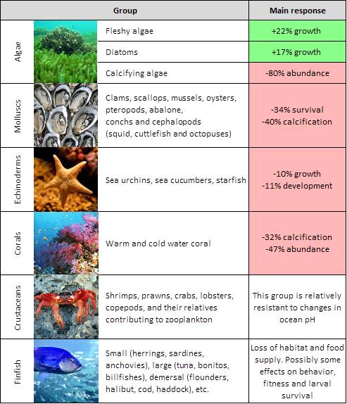
Hint for question 4:
Use the attached image (figure 5 in this website) and this mapping tool. Search for each species on the mapping tool to see the spatial global distribution.
Further Reading#
Understanding Ocean Acidification”, NOAA (https://www.fisheries.noaa.gov/insight/understanding-ocean-acidification)
“Ocean acidification and its effects”, CoastAdapt (https://coastadapt.com.au/ocean-acidification-and-its-effects)
“Scientists Pinpoint How Ocean Acidification Weakens Coral Skeletons”, WHOI (https://www.whoi.edu/press-room/news-release/scientists-identify-how-ocean-acidification-weakens-coral-skeletons/)
“Ocean acidification and reefs”, Smithonian Tropical Research Institute (https://stri.si.edu/story/ocean-acidification-and-reefs)
Henry, Joseph, Joshua Patterson, and Lisa Krimsky. 2020. “Ocean Acidification: Calcifying Marine Organisms: FA220, 3/2020”. EDIS 2020 (2):4. https://doi.org/10.32473/edis-fa220-2020.
Resources#
This tutorial uses data from the simulations conducted as part of the CMIP6 multi-model ensemble.
For examples on how to access and analyze data, please visit the Pangeo Cloud CMIP6 Gallery
For more information on what CMIP is and how to access the data, please see this page.