![]()

Bonus Tutorial 6: Radiative-Convective Equilibrium#
Week 1, Day 5, Introduction to Climate Modeling
Content creators: Jenna Pearson and Brian E. J. Rose
Content reviewers: Mujeeb Abdulfatai, Nkongho Ayuketang Arreyndip, Jeffrey N. A. Aryee, Younkap Nina Duplex, Will Gregory, Paul Heubel, Zahra Khodakaramimaghsoud, Peter Ohue, Abel Shibu, Derick Temfack, Yunlong Xu, Peizhen Yang, Ohad Zivan, Chi Zhang
Content editors: Abigail Bodner, Paul Heubel, Brodie Pearson, Ohad Zivan, Chi Zhang
Production editors: Wesley Banfield, Paul Heubel, Jenna Pearson, Konstantine Tsafatinos, Chi Zhang, Ohad Zivan
Our 2024 Sponsors: CMIP, NFDI4Earth
Tutorial Objectives#
Estimated timing of tutorial: 20 minutes
Note that this and the two previous tutorials contain solely Bonus content that serves experienced participants and for later investigation of 0- and 1-dimensional models after the course. Please check out these tutorials after finishing Tutorial 7-8 successfully.
Building on the understanding of a one-dimensional radiative balance model from the previous tutorial, in this tutorial you will learn about radiative-convective-equilibrium. Much of the code shown here was taken from The Climate Laboratory by Brian E. J. Rose. You are encouraged to visit this website for more tutorials and background on these models.
By the end of this tutorial you will be able to:
Implement a radiative-convective equilibrium model using the python package
climlab.Understand how this model builds off the one-dimensional radiative balance model used in the previous tutorials.
Setup#
# installations ( uncomment and run this cell ONLY when using google colab or kaggle )
# note the conda install takes quite a while, but conda is REQUIRED to properly download the
# dependencies (that are not just python packages)
# !pip install condacolab &> /dev/null
# import condacolab
# condacolab.install()
# !mamba install -c anaconda cftime xarray numpy &> /dev/null # for decoding time variables when opening datasets
# !mamba install -c conda-forge metpy climlab &> /dev/null
# imports
# google colab users, if you get an xarray error, please run this cell again
import xarray as xr # used to manipulate data and open datasets
import numpy as np # used for algebra/arrays
import climlab # one of the models we are using
import matplotlib.pyplot as plt # used for plotting
import metpy # used to make Skew T Plots of temperature and pressure
from metpy.plots import SkewT # plotting function used widely in climate science
import pooch
import os
import tempfile
from IPython.display import HTML
from matplotlib import animation
/opt/hostedtoolcache/Python/3.9.19/x64/lib/python3.9/site-packages/climlab/radiation/cam3.py:46: UserWarning: Cannot import and initialize compiled Fortran extension, CAM3 module will not be functional.
warnings.warn('Cannot import and initialize compiled Fortran extension, CAM3 module will not be functional.')
/opt/hostedtoolcache/Python/3.9.19/x64/lib/python3.9/site-packages/climlab/convection/emanuel_convection.py:14: UserWarning: Cannot import EmanuelConvection fortran extension, this module will not be functional.
warnings.warn('Cannot import EmanuelConvection fortran extension, this module will not be functional.')
Figure settings#
Show code cell source
# @title Figure settings
import ipywidgets as widgets # interactive display
%config InlineBackend.figure_format = 'retina'
plt.style.use(
"https://raw.githubusercontent.com/neuromatch/climate-course-content/main/cma.mplstyle"
)
Helper functions#
Show code cell source
# @title Helper functions
def pooch_load(filelocation=None, filename=None, processor=None):
shared_location = "/home/jovyan/shared/Data/tutorials/W1D4_ClimateModeling" # this is different for each day
user_temp_cache = tempfile.gettempdir()
if os.path.exists(os.path.join(shared_location, filename)):
file = os.path.join(shared_location, filename)
else:
file = pooch.retrieve(
filelocation,
known_hash=None,
fname=os.path.join(user_temp_cache, filename),
processor=processor,
)
return file
Plotting Functions#
Show code cell source
# @title Plotting Functions
# make the videos at the end of the tutorial
plt.rcParams["animation.html"] = "jshtml"
# these three functions are used to make videos at the end of the tutorial
def initial_figure(model):
with plt.ioff(): # will hide the inital figure which will plot separate from the video otherwise
fig = plt.figure(figsize=(6, 6))
lines = []
skew = SkewT(fig, rotation=30)
# plot the observations
skew.plot(
Tglobal.level,
Tglobal,
color="black",
linestyle="-",
linewidth=2,
label="Observations",
)
lines.append(
skew.plot(
model.lev,
model.Tatm - climlab.constants.tempCtoK,
linestyle="-",
linewidth=2,
color="C0",
label="RC model (all gases)",
)[0]
)
skew.ax.legend()
skew.ax.set_ylim(1050, 10)
skew.ax.set_xlim(-60, 75)
# Add the relevant special lines
skew.plot_dry_adiabats(linewidth=1.5, label="dry adiabats")
# skew.plot_moist_adiabats(linewidth=1.5, label = 'moist adiabats')
skew.ax.set_xlabel("Temperature ($^\circ$C)", fontsize=14)
skew.ax.set_ylabel("Pressure (hPa)", fontsize=14)
lines.append(
skew.plot(
1000,
model.Ts - climlab.constants.tempCtoK,
"o",
markersize=8,
color="C0",
)[0]
)
return fig, lines
def animate(day, model, lines):
lines[0].set_xdata(np.array(model.Tatm) - climlab.constants.tempCtoK)
lines[1].set_xdata(np.array(model.Ts) - climlab.constants.tempCtoK)
# lines[2].set_xdata(np.array(model.q)*1E3)
# lines[-1].set_text('Day {}'.format(int(model.time['days_elapsed'])))
# This is kind of a hack, but without it the initial frame doesn't appear
if day != 0:
model.step_forward()
return lines
# to setup the skewT and plot observations
def make_basic_skewT():
fig = plt.figure(figsize=(9, 9))
skew = SkewT(fig, rotation=30)
skew.plot(
Tglobal.level,
Tglobal,
color="black",
linestyle="-",
linewidth=2,
label="Observations",
)
skew.ax.set_ylim(1050, 10)
skew.ax.set_xlim(-90, 45)
# Add the relevant special lines
# skew.plot_dry_adiabats(linewidth=1.5, label = 'dry adiabats')
# skew.plot_moist_adiabats(linewidth=1.5, label = 'moist adiabats')
# skew.plot_mixing_lines()
skew.ax.legend()
skew.ax.set_xlabel("Temperature (degC)", fontsize=14)
skew.ax.set_ylabel("Pressure (hPa)", fontsize=14)
return skew
# to setup the skewT and plot observations
def make_skewT():
fig = plt.figure(figsize=(9, 9))
skew = SkewT(fig, rotation=30)
skew.plot(
Tglobal.level,
Tglobal,
color="black",
linestyle="-",
linewidth=2,
label="Observations",
)
skew.ax.set_ylim(1050, 10)
skew.ax.set_xlim(-90, 45)
# Add the relevant special lines
skew.plot_dry_adiabats(linewidth=1.5, label="dry adiabats")
# skew.plot_moist_adiabats(linewidth=1.5, label = 'moist adiabats')
# skew.plot_mixing_lines()
skew.ax.legend()
skew.ax.set_xlabel("Temperature (degC)", fontsize=14)
skew.ax.set_ylabel("Pressure (hPa)", fontsize=14)
return skew
# to add a model derived profile to the skewT figure
def add_profile(skew, model, linestyle="-", color=None):
line = skew.plot(
model.lev,
model.Tatm - climlab.constants.tempCtoK,
label=model.name,
linewidth=2,
)[0]
skew.plot(
1000,
model.Ts - climlab.constants.tempCtoK,
"o",
markersize=8,
color=line.get_color(),
)
skew.ax.legend()
Section 1: Reproducing Data from the Last Tutorial’s One-dimensional Radiative Equilibrium Model Using Climlab#
Please refer to the previous Bonus Tutorial 6 for a refresher if needed.
filename_sq = "cpl_1850_f19-Q-gw-only.cam.h0.nc"
url_sq = "https://osf.io/c6q4j/download/"
ds = xr.open_dataset(
pooch_load(filelocation=url_sq, filename=filename_sq)
) # ds = dataset
filename_ncep_air = "air.mon.1981-2010.ltm.nc"
url_ncep_air = "https://osf.io/w6cd5/download/"
ncep_air = xr.open_dataset(
pooch_load(filelocation=url_ncep_air, filename=filename_ncep_air)
) # ds = dataset
# take global, annual average of specific humidity
weight_factor = ds.gw / ds.gw.mean(dim="lat")
Qglobal = (ds.Q * weight_factor).mean(dim=("lat", "lon", "time"))
# use 'lev=Qglobal.lev' to create an identical vertical grid to water vapor data
mystate = climlab.column_state(lev=Qglobal.lev, water_depth=2.5)
radmodel = climlab.radiation.RRTMG(
name="Radiation (all gases)", # give our model a name
state=mystate, # give our model an initial condition
specific_humidity=Qglobal.values, # tell the model how much water vapor there is
albedo=0.25, # set the SURFACE shortwave albedo
timestep=climlab.constants.seconds_per_day, # set the timestep to one day (measured in seconds)
)
# need to take the average over space and time
# the grid cells are not the same size moving towards the poles, so we weight by the cosine of latitude to compensate for this
coslat = np.cos(np.deg2rad(ncep_air.lat))
weight = coslat / coslat.mean(dim="lat")
# global mean temperature from NCEP
Tglobal = (ncep_air.air * weight).mean(dim=("lat", "lon", "time"))
# take a single step forward until the diagnostics are updated and there is some energy imbalance
radmodel.step_forward()
# run the model to equilibrium (the difference between ASR and OLR is a very small number)
while np.abs(radmodel.ASR - radmodel.OLR) > 0.001:
radmodel.step_forward()
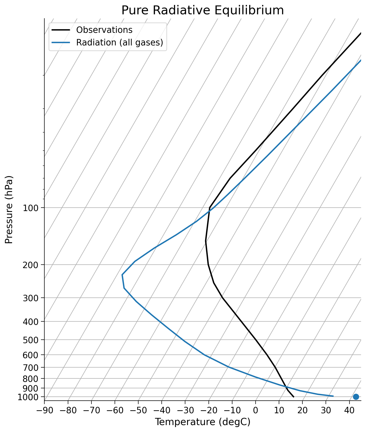
skew = make_basic_skewT()
add_profile(skew, radmodel)
skew.ax.set_title("Pure Radiative Equilibrium")
/opt/hostedtoolcache/Python/3.9.19/x64/lib/python3.9/site-packages/xarray/coding/times.py:995: SerializationWarning: Unable to decode time axis into full numpy.datetime64 objects, continuing using cftime.datetime objects instead, reason: dates out of range
dtype = _decode_cf_datetime_dtype(data, units, calendar, self.use_cftime)
/opt/hostedtoolcache/Python/3.9.19/x64/lib/python3.9/site-packages/xarray/coding/times.py:170: SerializationWarning: Ambiguous reference date string: 1-1-1 00:00:0.0. The first value is assumed to be the year hence will be padded with zeros to remove the ambiguity (the padded reference date string is: 0001-1-1 00:00:0.0). To remove this message, remove the ambiguity by padding your reference date strings with zeros.
warnings.warn(warning_msg, SerializationWarning)
/opt/hostedtoolcache/Python/3.9.19/x64/lib/python3.9/site-packages/xarray/core/indexing.py:557: SerializationWarning: Unable to decode time axis into full numpy.datetime64 objects, continuing using cftime.datetime objects instead, reason: dates out of range
array = array.get_duck_array()
Text(0.5, 1.0, 'Pure Radiative Equilibrium')
Section 2: Radiative-Convective Equilibrium#
From the plot you just made, one of the largest differences between observations and the pure radiation model with all gases lies in the lower atmosphere, where the surface air temperature is 20 degrees too warm and the 200 hPa pressure surface is 40 degrees too cold. What could be the issue?
One thing we have not included in our model yet is dynamics (motion of the air). The model’s temperature profile is what’s known as statically unstable (note this definition of stability is different than that used in the previous tutorials).
Here static means not due to wind, and unstable means the atmosphere wants to adjust to a different state because the surface air is relatively light and wants to rise into upper layers of the atmosphere. As the air rises, it creates convective turbulence (similar to boiling water, where convective circulation is introduced by heating water from below). The rising air, and the resultant turbulence, mixes the atmospheric column. This mixing often occurs across the troposphere, which is roughly the lowest \(10 \text{ km}\) of the atmosphere. Most of the weather we experience lies in the troposphere.
When air rises adiabatically, it expands and cools due to the lower pressure. The rate of cooling depends on whether the air is saturated with water vapor. When rising air is unsaturated, it cools following the dry adiabats. If the air saturates, it cools at a lesser rate denoted by the moist adiabats (we did not have time to discuss these moisture effects in the mini-lecture).
To identify unstable atmospheric layers, let’s take another look at the SkewT plot, but this time we will plot the dry adiabats. We can then compare the rates of cooling of our model to these adiabats.
skew = make_skewT()
add_profile(skew, radmodel)
skew.ax.set_title("Pure Radiative Equilibrium")
Text(0.5, 1.0, 'Pure Radiative Equilibrium')
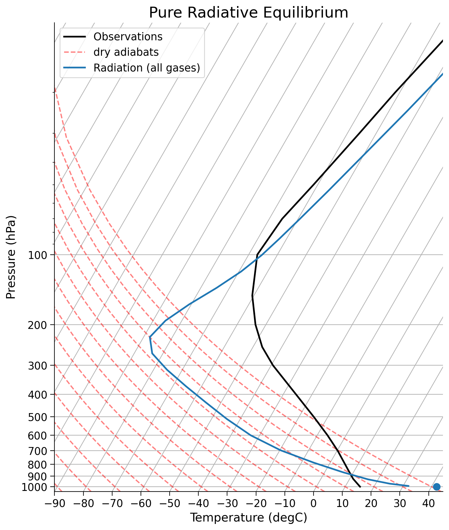
Near the surface, the reanalysis temperature profile is steeper than the dry adiabats. In these layers vertical motion is inhibited, and the surface conditions are considered stable. However, the model profile is shallower than the dry adiabats. In the model, the surface air is statically unstable, which would lead to convective mixing if this physical process was included in the model (the model currently only includes radiative processes). In this tutorial we will see whether including convective mixing in our model can bring the model closer to the reanalysis temperature profile.
To build a radiative-convective model we can take the radiative model we have already made and couple it to a convective model. Here the term couple implies there is communication between the models such that their effects are both incorporated into the final product, which in our case is the temperature profile.
# restate the model here for ease of coding
# make a model on same vertical domain as the water vapor data
mystate = climlab.column_state(lev=Qglobal.lev, water_depth=2.5)
# create the radiation model
rad = climlab.radiation.RRTMG(
name="Radiation (net)",
state=mystate,
specific_humidity=Qglobal.values,
timestep=climlab.constants.seconds_per_day,
albedo=0.25, # surface albedo, tuned to give reasonable ASR for reference cloud-free model
)
# create the convection model
conv = climlab.convection.ConvectiveAdjustment(
name="Convection",
state=mystate,
adj_lapse_rate=6.5, # the adiabatic lapse rate of the atmopshere
timestep=rad.timestep, # same timestep as radiation model
)
# couple the two components
rcm = climlab.couple([rad, conv], name="Radiative-Convective Model")
Now let’s run the radiation part to equilibrium, which should give us the same profile as in the previous section. Once we get this radiative equilibrium profile we will add convective mixing physics to the model and continue running it until it reaches radiative-convective equilibrium.
The new model does not actually resolve the actual vertical motion and mixing that occurs in convection. Instead, the model includes a parameterization for convection which automatically mixes regions of the atmospheric column that are statically unstable.
# run JUST the radiative component to equilibrium
for n in range(1000):
rcm.subprocess["Radiation (net)"].step_forward()
# compute diagnostics
rcm.compute_diagnostics()
# plot the resulting profile (our initial condition once we turn on the physics)
fig, lines = initial_figure(rcm)
# this animation can take a while
animation.FuncAnimation(fig, animate, 50, fargs=(rcm, lines))
Adding convective mixing to the initially unstable temperature profile leads to an instant mixing of air throughout the lower atmosphere, moving the profile toward the observations. The balance at play is between radiative processes that warm the surface and cool the troposphere (lower atmosphere) as well as convection which moves heat away from the surface, leading to a colder surface and warmer troposphere. Note the differences in surface versus tropospheric temperatures in the new versus old equilibrium profiles.
Questions 2: Climate Connection#
The static instability was removed in the first time step! In reality, which process do you think changes temperature faster, convection or radiation?
What do you think the next step would be to move towards a more realistic climate model?
Coding Exercises#
Recreate the video above except using an isothermal atmosphere (uniform temperature profile) set to the surface temperature
rcm.state.Ts. Does the equilbrium profile look any different than the one you made before?
# set initial temperature profile to be the surface temperature (isothermal)
rcm.state.Tatm[:] = rcm.state.Ts
# compute diagnostics
_ = ...
# plot initial data
fig, lines = initial_figure(rcm)
# make animation - this animation can take a while
# animation.FuncAnimation(fig, animate, 50, fargs=(rcm, lines))
Summary#
In this tutorial, you explored the concept of radiative-convective equilibrium, learning to implement a Python model using the climlab package. You learned the limitations of a pure radiation model and the necessity to include atmospheric dynamics such as convection. Through coupling a radiation model with a convective model, you have simulated a more realistic atmospheric temperature profile. Even though the model does not directly resolve the vertical motion during convection, it incorporates a parameterization to automatically account for mixing in statically unstable regions. By the end of the tutorial, you could comprehend how this model expands on the previous energy balance models from tutorials 1-4.
Resources#
Data from this tutorial can be accessed for specific humidity here and reanalysis temperature here.
Useful links:
The Climate Laboratory by Brian E. J. Rose,