![]()

Tutorial 1: Radiation and the Greenhouse Effect#
Week 1, Day 5, Introduction to Climate Modeling
Content creators: Jenna Pearson and Brian E. J. Rose
Content reviewers: Mujeeb Abdulfatai, Nkongho Ayuketang Arreyndip, Jeffrey N. A. Aryee, Dionessa Biton, Younkap Nina Duplex, Will Gregory, Paul Heubel, Zahra Khodakaramimaghsoud, Peter Ohue, Abel Shibu, Derick Temfack, Yunlong Xu, Peizhen Yang, Chi Zhang, Ohad Zivan
Content editors: Brodie Pearson, Abigail Bodner, Paul Heubel, Ohad Zivan, Chi Zhang
Production editors: Wesley Banfield, Paul Heubel, Jenna Pearson, Konstantine Tsafatinos, Chi Zhang, Ohad Zivan
Our 2024 Sponsors: CMIP, NFDI4Earth
Tutorial Objectives#
Estimated timing of tutorial: 30 minutes
In this tutorial, students will learn about blackbody radiation and greenhouse models for energy emitted from Earth.
By the end of this tutorial students will be able to:
Understand what an emission temperature is, and how to find it given observed outgoing longwave radiation.
Modify the blackbody radiation model to include the greenhouse effect.
Setup#
# imports
import matplotlib.pyplot as plt
import numpy as np
Figure settings#
Show code cell source
# @title Figure settings
import ipywidgets as widgets  # interactive display

%config InlineBackend.figure_format = 'retina'
plt.style.use(
    "https://raw.githubusercontent.com/neuromatch/climate-course-content/main/cma.mplstyle"
)
Video 1: Speaker Introduction#
Section 1: A Radiating Earth#
Section 1.1: Planck’s Law#
All objects with a temperature emit electromagnetic radiation. This energy travels through space in the form of waves. In the lecture we discussed that blackbody radiation is a model of how Earth loses radiative energy to space. Although this is not a perfect model for Earth, we will use it as a basis to understand Earth’s energy balance throughout tutorials 1-4. If we suppose Earth behaves as a perfect blackbody, then it emits energy at all wavelengths according to Planck’s Law:
where \(h = 6.626075 \times 10^{-34} \text{ J s}\) is Planck’s constant, \(c= 2.99792 \times 10^8 \text{ m s}^{-1}\) is the speed of light, and \(\kappa = 1.3804 \times 10^{23} \text{ W K}^{-1}\) is Boltzmann’s constant.
Interactive Demo 1.1#
This interactive demo will allow you to visualize how the blackbody curve changes as Earth warms and cools relative to its current surface temperature of about 288 K. Use the slide bar to adjust the emission temperature. Give the code a few seconds to replot before choosing a new temperature.
No need to worry about understanding the code here - this is conceptual.
Make sure you execute this cell to enable the widget! Please run this cell twice to be able to use the slides bar
Show code cell source
# @markdown Make sure you execute this cell to enable the widget! Please run this cell **twice** to be able to use the slides bar
import holoviews as hv
import panel as pn
hv.extension("bokeh")

# define constants used in Planck's Law
h = 6.626075e-34  # J s
c = 2.99792e8  # m s^-1
k = 1.3804e-23  # W K^-1


# define the function for Planck's Law depedent on wavelength (lambda) and temeprature (T)
def planck(wavelength, temperature):
    a = 2.0 * h * c**2
    b = h * c / (wavelength * k * temperature)
    intensity = a / ((wavelength**5) * (np.exp(b) - 1.0))

    lpeak = (2.898 * 1e-3) / temperature

    return intensity


def update_plot(emiss_temp):
    # generate x-axis in increments from 1um to 100 micrometer in 1 nm increments
    # starting at 1 nm to avoid wav = 0, which would result in division by zero.
    wavelengths = np.arange(1e-6, 50e-6, 1e-9)

    # get the blackbody curve and peak emission wavelength for 288 K
    intensity288 = planck(wavelengths, 288)

    # get the blackbody curve and peak emission wavelength for selected temperature
    intensity = planck(wavelengths, emiss_temp)

    #     # get the intensity at peak wavelength to limit the lines
    #     Ipeak,_ = planck(lpeak,emission_temperature)
    #     Ipeak288,_ = planck(lpeak288,288)

    # curves output
    vary = zip(wavelengths * 1e6, intensity)
    init_val = zip(wavelengths * 1e6, intensity288)

    # Specified individually
    list_of_curves = [
        hv.Curve(init_val, label="T=288K").opts(ylim=(0, 1.0e7)),
        hv.Curve(vary, label="T=" + str(emiss_temp) + "K").opts(ylim=(0, 1.0e7)),
    ]

    bb_plot = hv.Overlay(list_of_curves).opts(
        height=300,
        width=600,
        xlabel="Wavelength (μm)",
        ylabel="B(λ,T) (W/(m³ steradian)",
        title="Spectral Radiance",
    )

    return bb_plot


emiss_temp_widget = pn.widgets.IntSlider(
    name="Emission Temperature", value=288, start=250, end=300
)
bound_plot = pn.bind(update_plot, emiss_temp=emiss_temp_widget)

pn.Row(emiss_temp_widget, bound_plot)


Questions 1.1: Climate Connection#
Recall from Tutorial 1 on Week 1 Day 3 the electromagnetic spectrum (shown below), which displays the different wavelengths of electromagnetic energy. According to our model and noting that 1 micrometer = \(10^{-6}\) meters, with a surface temperature of 288 K what type of radiation does Earth primarily emit at?
 Diagram of the Electromagnetic Spectrum. (Credit: Wikipedia)
Section 1.2: The Stefan-Boltzmann Law#
If we integrate Planck’s Law over all wavelengths and outward angles of emission, the total outgoing longwave radiation (OLR) for a given emission temperature (\(\mathbf{T}\)) follows the Stefan-Boltzmann Law.
Where the Stefan-Boltzmann constant is \(\sigma = 5.67 \times 10^{-8}\text{ W m}^{-2} \text{ K}^{-4}\).
Rearranging the equation above, we can solve for the emission temperature of Earth, \(T\).
Using \(OLR = 239\text{ W m}^{-2}\) we can calculate the value of \(T\):
# define the Stefan-Boltzmann Constant, noting we are using 'e' for scientific notation
sigma = 5.67e-8  # W m^-2 K^-4

# define the outgoing longwave radiation based on observations from the IPCC AR6 Figure 7.2
OLR = 239  # W m^-2

# plug into equation
T = (OLR / sigma) ** (1 / 4)

# display answer
print("Emission Temperature: ", T, "K or", T - 273, "°C")
Emission Temperature: 254.80251510194708 K or -18.19748489805292 °C
Questions 1.2: Climate Connection#
How does this compare to the actual global mean surface temperature of \(~288 \text{ K} / 15\text{°C}\)?
Using \(T = 288 \text{ K}\) would you expect the corresponding outgoing longwave radiation to be higher or lower than the observed \(239 \text{ W m}^{-2}\)?
What could be accounted for in this model to make it more realistic?
Coding Exercises 1.2#
By modifying the code above and solving for OLR, find the outgoing longwave radiation expected for the observed surface temperature of \(288 \text{ K}\). This should help you answer Question 2 above.
# define the Stefan-Boltzmann Constant, noting we are using 'e' for scientific notation
sigma = ...

# define the global mean surface temperature based on observations
T = ...

# plug into equation
OLR = ...

# display answer
print("OLR: ", OLR, "W m^2")
OLR: Ellipsis W m^2
Section 2: The Greenhouse Effect#
Section 2.1: About greenhouse gases#
The expected surface temperature using the blackbody radiation model is much colder than we observe it to be. In this model, we assumed there is nothing that lies between Earth’s surface and space that interacts with Earth’s emitted radiation. From the initial lecture on the global energy budget we know this is not true. Earth has an atmosphere, and within it are many gases that interact with radiation in the infrared range at which Earth primarily emits. The effect of these gases on radiation, called the greenhouse effect, is what warms earth to a habitable temperature.
The gases that are responsible for this (carbon dioxide, water vapor, methane, ozone, nitrous oxide, and chloroflourocarbons) are termed greenhouse gases, and are all trace gases present in very low concentrations in Earth’s atmosphere. Anthropogenic climate change is caused to a large extent by increased concentrations of many of these trace gases due to emissions from human activities.
The figure below shows the contributions to the global surface air temperature change relative to 1750. We can see that all of the greenhouse gases have contributed positively, that is towards warming Earth. Also, note that the total curve tracks the volcano curve quite well until around the 1850s when industrialization took hold. The total and volcanic curves begin to deviate here, and after the mid-1900s the total curve begins tracking the total anthropogenic curve instead.
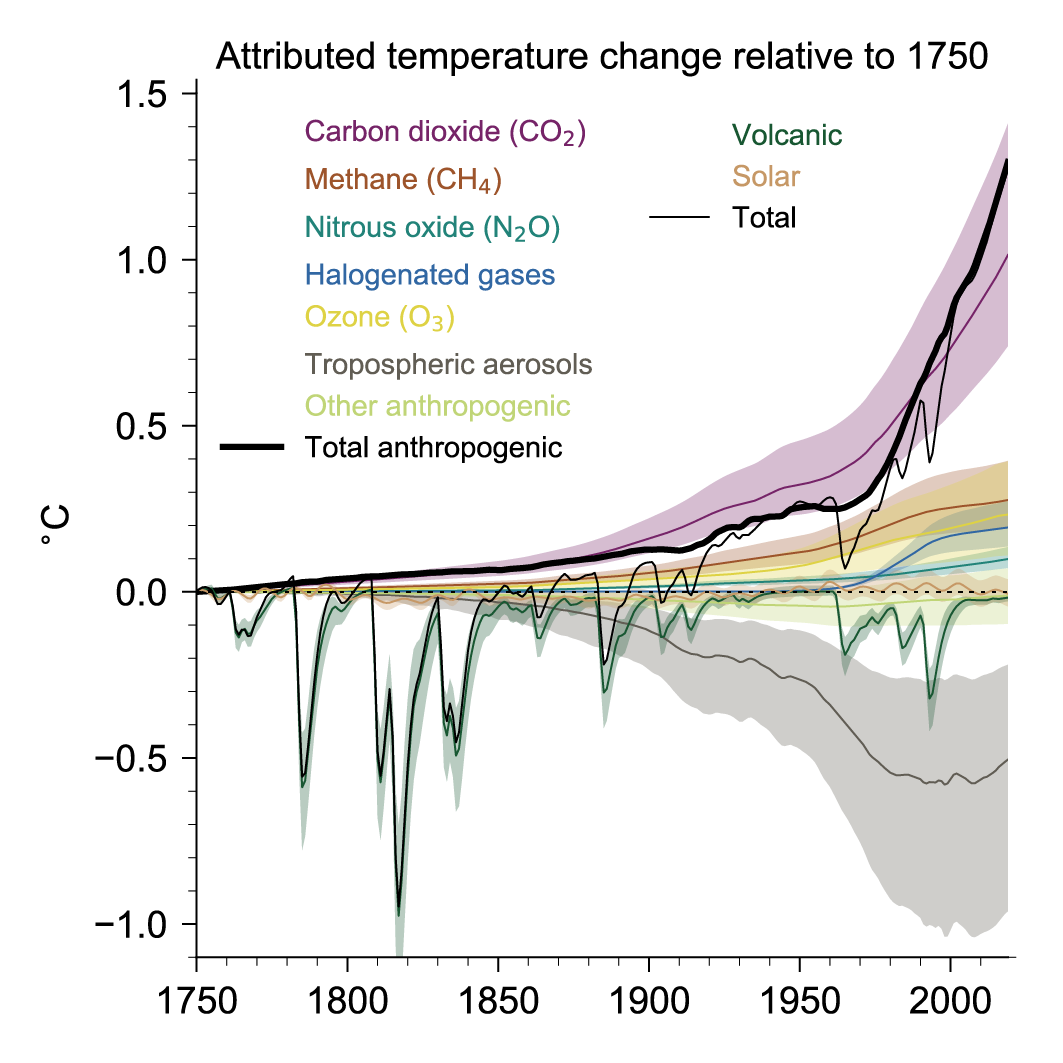
Figure 7.8 | Attributed global surface air temperature change (GSAT) from 1750 to 2019 produced using the two-layer emulator (Supplementary Material 7.SM.2), forced with ERF derived in this chapter (displayed in Figure 2.10) and climate response constrained to assessed ranges for key climate metrics described in Cross-Chapter Box 7.1. The results shown are the medians from a 2237-member ensemble that encompasses uncertainty in forcing and climate response (year-2019 best estimates and uncertainties are shown in Figure 7.7 for several components). Temperature contributions are expressed for carbon dioxide (CO2), methane (CH4), nitrous oxide (N2O), other well-mixed greenhouse gases (WMGHGs), ozone (O3), aerosols, and other anthropogenic forcings, as well as total anthropogenic, solar, volcanic, and total forcing. Shaded uncertainty bands show very likely (5–95%) ranges. Further details on data sources and processing are available in the chapter data table (Table 7.SM.14). (Credit IPCC)
Section 2.2: A simple greenhouse model#
This section draws content from The Climate Laboratory by Brian E. J. Rose.
As shown above, greenhouse gases are incredibly important for regulating Earth’s energy balance and temperature. A first approach is to model the greenhouse effect on outgoing longwave radiation (OLR) to space by adding a transmissivity coefficient. The transmissivity coeficient (\(\mathbf{\tau}\)) is the fraction of the radiation emitted from Earth that actually makes it to space. This coefficient \(\mathbf{\tau}\) is a number that lies between 0 and 1, and represents the effects of all the greenhouse gases on radiation, rather than including them explicity in the model. This approach is called a parametrization.
Applying this to the original model for blackbody radiation, the modified model is
Using \(OLR = 239 \text{ W m}^{-2}\) and \(T = 288 \text{ K}\), we can estimate \(\tau\).
# define the Stefan-Boltzmann Constant, noting we are using 'e' for scientific notation
sigma = 5.67e-8  # W m^-2 K^-4

# define the outgoing longwave radiation based on observations from the IPCC AR6 Figure 7.2
OLR = 239  # W m^-2

# define the emission temperature based on observtions of global mean surface temperature
T = 288  # K

# plug into equation
tau = OLR / (sigma * T**4)  # unitless number between 0 and 1

# display answer
print("Transmissivity Coefficient: ", tau)
Transmissivity Coefficient: 0.6126957827090973
Questions 2.2: Climate Connection#
For a generic planet, what could be said about the planet’s atmosphere when \(\tau\) is close to 1? Close to 0? Use the OLR seen at the top of the atmosphere in your answer.
In terms of energy received from the sun, what does only modifying the OLR to account for the greenhouse effect imply? Are there any greenhouse gases you think would make this implication problematic?
Is there any other part of the atmosphere aside from greenhouse gases that we have not discussed that would also affect \(\tau\)?
Coding Exercises 2.2#
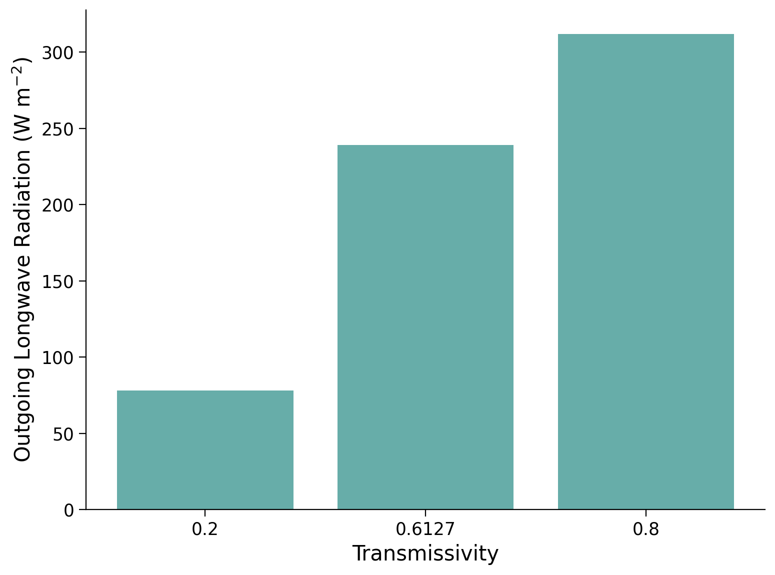
Using list comprehension, calculate the OLR for three values of \(\tau = 0.2,0.6114,0.8\). Then plot this on a bar chat to compare. This should help you answer question 1 above. Hint: what is list comprehension?
# define the Stefan-Boltzmann Constant, noting we are using 'e' for scientific notation
sigma = ...

# define the emission temperature based on observtions of global mean surface temperature
T = ...

# define values of tau
tau = ...

# get values of OLR from tau using list comprehension
OLR = ...

# convert tau to list of strings using list comprehension so we can create a categorical plot
tau = ...

fig, ax = plt.subplots()
_ = ...
ax.set_xlabel("Transmissivity")
ax.set_ylabel("Outgoing Longwave Radiation (W m$^{-2}$)")
Text(0, 0.5, 'Outgoing Longwave Radiation (W m$^{-2}$)')
Example output:
Bonus Section 3: An Additional Exercise on Blackbody Radiation#
Want to explore the concept of Blackbody radiation a bit more? Try this additional exercise! Be aware that this will take at least another 15 minutes.
Instructions#
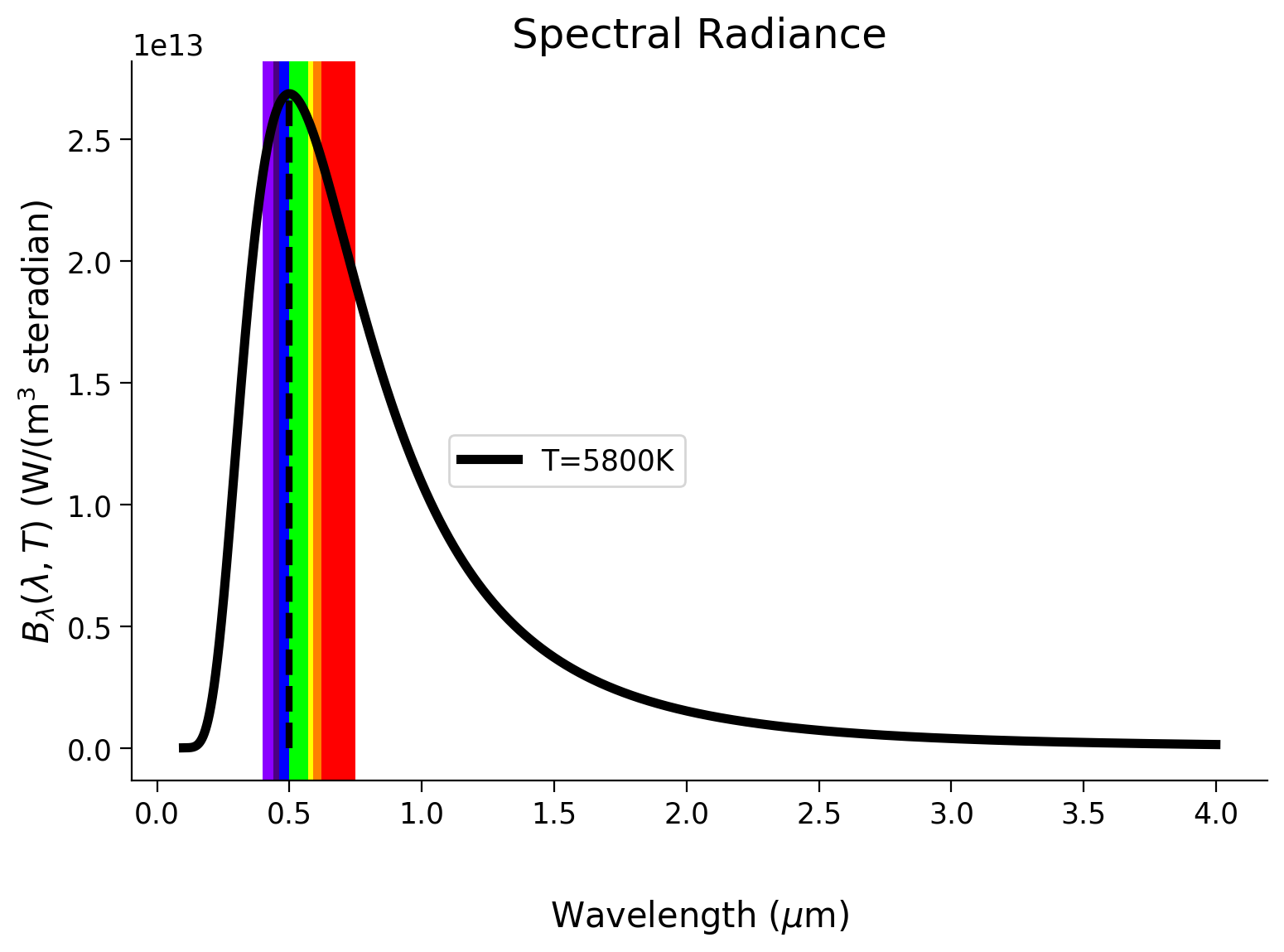
By defining a function for Planck’s Law, plot the blackbody radiation curve for the sun, assuming an emission temperature of \(5800 \text{ K}\). Underlay an approximation of the visible range from the electromagnetic spectrum. This exercise should help you understand why we see in color as well as why the sun’s radiation headed towards Earth is called incoming shortwave radiation.
# define the emission temperature of the sun
T_sun = ...


# define constants used in Planck's Law
h = 6.626075e-34  # J s
c = 2.99792e8  # m s^-1
k = 1.3804e-23  # W K^-1


# define the function for Planck's Law that returns the intensity as well
# as the peak wavelength defined by Wien's Law
def planck(wavelength, temperature):
    ...
    intensity = ...
    lpeak = ...
    return intensity, lpeak


# generate x-axis in increments from 1um to 100 micrometer in 1 nm increments
# starting at 1 nm to avoid wav = 0, which would result in division by zero.
wavelengths = np.arange(1e-7, 4e-6, 1e-9)

# intensity and peak radiating wavelength at different temperatures
intensity, lpeak = planck(wavelengths, T_sun)

# get the intensity at peak wavelength to limit the lines
Ipeak, _ = planck(lpeak, T_sun)

# plot an approximation of the visible range by defining a dictionary with
# wavelength ranges and colors
rainbow_dict = {
    (0.4, 0.44): "#8b00ff",
    (0.44, 0.46): "#4b0082",
    (0.46, 0.5): "#0000ff",
    (0.5, 0.57): "#00ff00",
    (0.57, 0.59): "#ffff00",
    (0.59, 0.62): "#ff7f00",
    (0.62, 0.75): "#ff0000",
}

fig, ax = plt.subplots()

for wv_range, rgb in rainbow_dict.items():
    ax.axvspan(*wv_range, color=rgb, ec="none")

# add in wiens law
_ = ...

# plot intensity curve
_ = ...

ax.set_xlabel("Wavelength ($\mu$m)", labelpad=30)
ax.set_ylabel("$B_\lambda(\lambda,T)$ (W/(m$^3$ steradian)")

ax.set_title("Spectral Radiance")

# add legend
ax.legend(bbox_to_anchor=(0.5, 0.5))
/tmp/ipykernel_112899/1991545529.py:59: UserWarning: No artists with labels found to put in legend.  Note that artists whose label start with an underscore are ignored when legend() is called with no argument.
  ax.legend(bbox_to_anchor=(0.5, 0.5))
<matplotlib.legend.Legend at 0x7f9eb8ac2b20>
Example output:
Summary#
In this tutorial, we’ve learned about the principles of blackbody and greenhouse radiation models, which are crucial to understanding Earth’s energy emission. We explored the concept of emission temperature and how it’s calculated using observed outgoing longwave radiation. We discovered that the simple blackbody model needs to be augmented by considering the greenhouse effect to accurately represent Earth’s observed surface temperature. This led us to incorporate the transmissivity coefficient, a representation of greenhouse gases’ impact, into our model.