Tutorial 3: Opening and Plotting netCDF Data

Tutorial 3: Opening and Plotting netCDF Data#

Week 1, Day 1, Climate System Overview

Content creators: Sloane Garelick, Julia Kent

Content reviewers: Katrina Dobson, Younkap Nina Duplex, Danika Gupta, Maria Gonzalez, Will Gregory, Nahid Hasan, Paul Heubel, Sherry Mi, Beatriz Cosenza Muralles, Jenna Pearson, Agustina Pesce, Chi Zhang, Ohad Zivan

Content editors: Paul Heubel, Jenna Pearson, Chi Zhang, Ohad Zivan

Production editors: Wesley Banfield, Paul Heubel, Jenna Pearson, Konstantine Tsafatinos, Chi Zhang, Ohad Zivan

Our 2024 Sponsors: CMIP, NFDI4Earth

#

Pythia credit: Rose, B. E. J., Kent, J., Tyle, K., Clyne, J., Banihirwe, A., Camron, D., May, R., Grover, M., Ford, R. R., Paul, K., Morley, J., Eroglu, O., Kailyn, L., & Zacharias, A. (2023). Pythia Foundations (Version v2023.05.01) https://zenodo.org/record/8065851

#

Tutorial Objectives#

Estimated timing of tutorial: 30 minutes

Many global climate datasets are stored as NetCDF (network Common Data Form) files. NetCDF is a file format for storing multidimensional variables such as temperature, humidity, pressure, wind speed, and direction. These types of files also include metadata that gives you information about the variables and the dataset itself.

In this tutorial, we will import atmospheric pressure and temperature data stored in a NetCDF file. We will learn how to use various attributes of Xarray to import, analyze, interpret, and plot the data.

Setup#

# installations ( uncomment and run this cell ONLY when using google colab or kaggle )
#!pip install pythia_datasets

# imports
import numpy as np
import xarray as xr
from pythia_datasets import DATASETS
import matplotlib.pyplot as plt

Figure Settings#

Video 1: Atmospheric Climate Systems#

Section 1: Opening netCDF Data#

Xarray is closely linked with the netCDF data model, and it even treats netCDF as a ‘first-class’ file format. This means that Xarray can easily open netCDF datasets. However, these datasets need to follow some of Xarray’s rules. One such rule is that coordinates must be 1-dimensional.

Here we’re getting the data from Project Pythia’s custom library of example data, which we already imported above with from pythia_datasets import DATASETS. The DATASETS.fetch() method will automatically download and cache (store) our example data file NARR_19930313_0000.nc locally.

filepath = DATASETS.fetch("NARR_19930313_0000.nc")

Downloading file 'NARR_19930313_0000.nc' from 'https://github.com/ProjectPythia/pythia-datasets/raw/main/data/NARR_19930313_0000.nc' to '/home/runner/.cache/pythia-datasets'.

Once we have a valid path to a data file that Xarray knows how to read, we can open it like this:

Questions 1#

What are the dimensions of this dataset?
How many climate variables are in this dataset?

Click for solution

Section 2: Plotting with Xarray#

Another major benefit of using labeled data structures is that they enable automated plotting with axis labels.

Section 2.1: Simple Visualization with `.plot()`#

Much like Pandas, Xarray includes an interface to Matplotlib that we can access through the .plot() method of every DataArray.

For quick and easy data exploration, we can just call .plot() without any modifiers:

prof.plot()

[<matplotlib.lines.Line2D at 0x7f3bec683070>]

../../../_images/f5264fc844bda75ca5838ee3e7d404a7ca9239deebb68a220709b32e2165f0ad.png

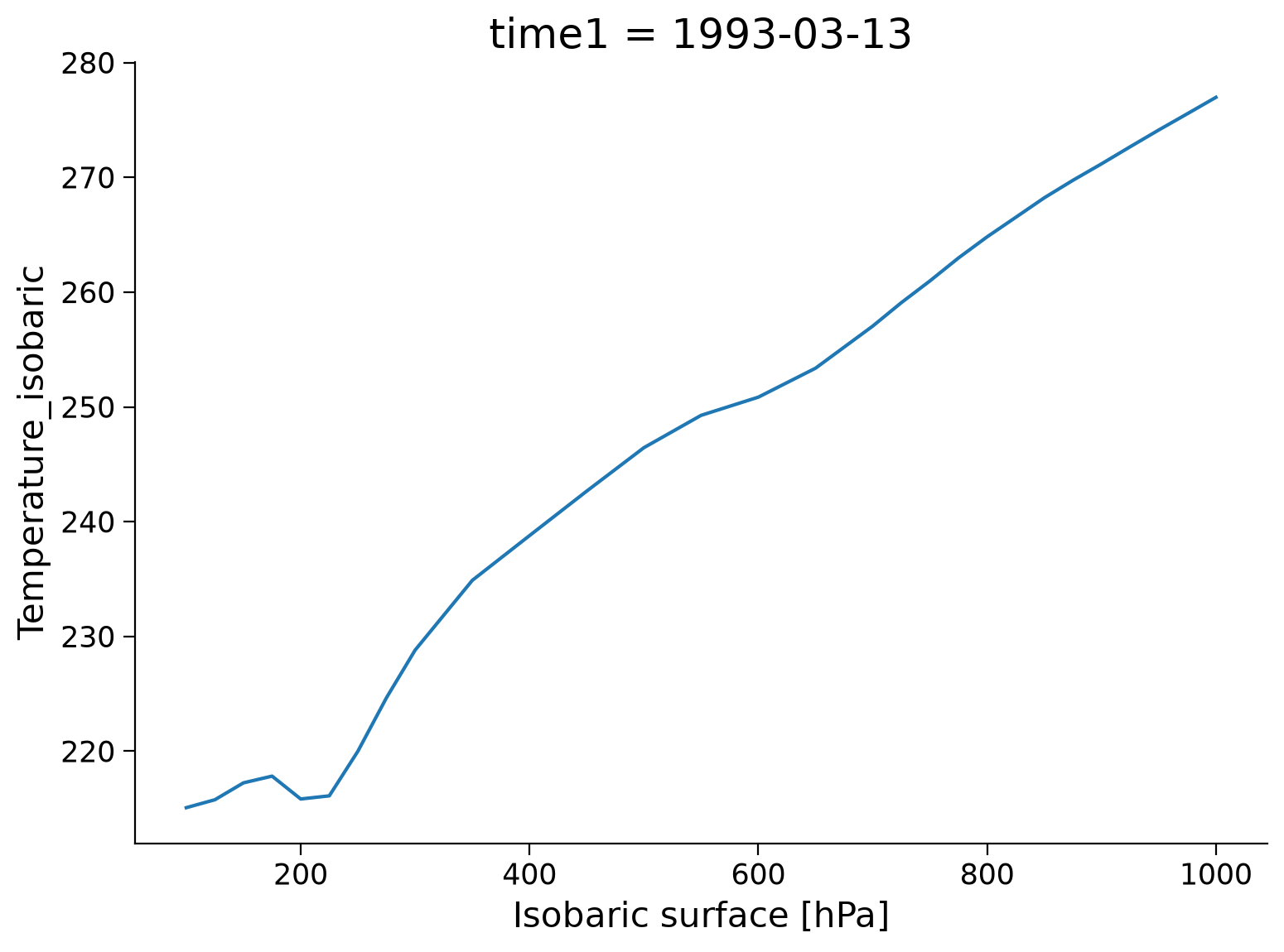
Here Xarray has generated a line plot of the temperature data against the coordinate variable isobaric. Also, the metadata are used to auto-generate axis labels and units.

Consider the following questions:

What isobaric pressure corresponds to Earth’s surface?
How does temperature change with increasing altitude in the atmosphere?

It might be a bit difficult to answer these questions with our current plot, so let’s try customizing our figure to present the data clearer.

Section 2.2: Customizing the Plot#

As in Pandas, the .plot() method is mostly just a wrapper to Matplotlib, so we can customize our plot in familiar ways.

In this air temperature profile example, we would like to make two changes:

swap the axes so that we have isobaric levels on the y-axis (vertical) of the figure (since isobaric levels correspond to altitude)
make pressure decrease upward in the figure so that up is up (since pressure decreases with altitude)

We can do this by adding a few keyword arguments to our .plot():

prof.plot(y="isobaric1", yincrease=False)

[<matplotlib.lines.Line2D at 0x7f3beca677c0>]

../../../_images/2e852e1f9a6e3cf1b28a12b481ab74887d41aac625ea2e92165a87dc2abab924.png

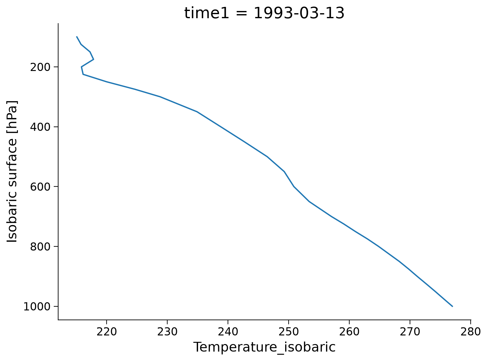
Questions 2.2#

What isobaric pressure corresponds to Earth’s surface?
Why do you think temperature generally decreases with height?

Click for solution

Section 2.3: Plotting 2D Data#

In the example above, the .plot() method produced a line plot.

What if we call .plot() on a 2D array? Let’s try plotting the temperature data from the 1000 hPa isobaric level (surface temperature) for all x and y values:

temps.sel(isobaric1=1000).plot()

<matplotlib.collections.QuadMesh at 0x7f3becaf9cd0>

../../../_images/a65082ca091bd8770737c1178df270cec350e8cae937420698959764ece86566.png

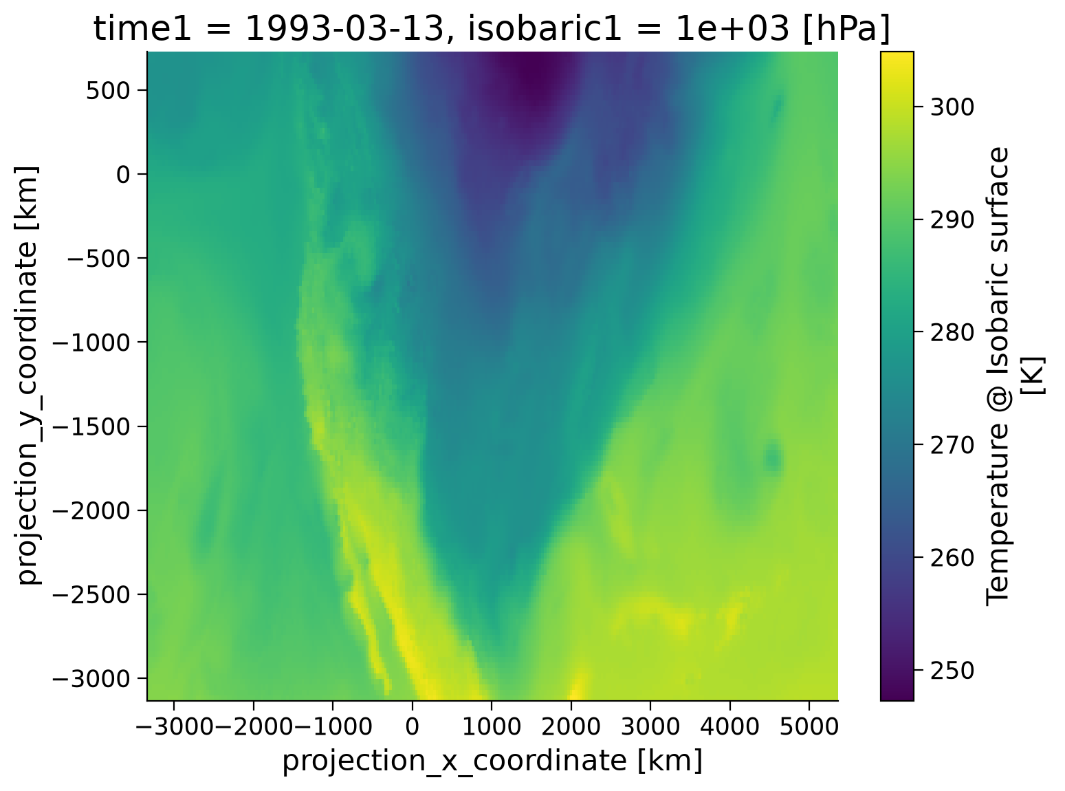
Xarray has recognized that the DataArray object calling the plot method has two coordinate variables, and generates a 2D plot using the .pcolormesh() method from Matplotlib.

In this case, we are looking at air temperatures on the 1000 hPa isobaric surface over North America. Note you could improve this figure further by using Cartopy to handle the map projection and geographic features.

Questions 2.3: Climate Connection#

The map you made shows the temperature across the United States at the 1000 hPa level of the atmosphere. How do you think temperatures at the 500 hPa level would compare? What might be causing the spatial differences in temperature seen in the map?

Click for solution

Summary#

Xarray brings the joy of Pandas-style labeled data operations to N-dimensional data. As such, it has become a central workhorse in the geoscience community for analyzing gridded datasets. Xarray allows us to open self-describing NetCDF files and make full use of the coordinate axes, labels, units, and other metadata. By utilizing labeled coordinates, our code becomes simpler to write, easier to read, and more robust.

Resources#

Code and data for this tutorial is based on existing content from Project Pythia.

Tutorial 3: Opening and Plotting netCDF Data

Contents

Tutorial 3: Opening and Plotting netCDF Data#

#

#

Tutorial Objectives#

Setup#

Figure Settings#

Video 1: Atmospheric Climate Systems#

Section 1: Opening netCDF Data#

Questions 1#

Section 1.1: Subsetting the `Dataset`#

Section 1.2: Aggregation Operations#

Section 2: Plotting with Xarray#

Section 2.1: Simple Visualization with `.plot()`#

Section 2.2: Customizing the Plot#

Questions 2.2#

Section 2.3: Plotting 2D Data#

Questions 2.3: Climate Connection#

Summary#

Resources#

Tutorial 3: Opening and Plotting netCDF Data

Contents

Tutorial 3: Opening and Plotting netCDF Data#

#

#

Tutorial Objectives#

Setup#

Figure Settings#

Video 1: Atmospheric Climate Systems#

Section 1: Opening netCDF Data#

Questions 1#

Section 1.1: Subsetting the Dataset#

Section 1.2: Aggregation Operations#

Section 2: Plotting with Xarray#

Section 2.1: Simple Visualization with .plot()#

Section 2.2: Customizing the Plot#

Questions 2.2#

Section 2.3: Plotting 2D Data#

Questions 2.3: Climate Connection#

Summary#

Resources#

Section 1.1: Subsetting the `Dataset`#

Section 2.1: Simple Visualization with `.plot()`#