![]()

Tutorial 7: Other Computational Tools in Xarray#
Week 1, Day 1, Climate System Overview
Content creators: Sloane Garelick, Julia Kent
Content reviewers: Katrina Dobson, Younkap Nina Duplex, Danika Gupta, Maria Gonzalez, Will Gregory, Nahid Hasan, Paul Heubel, Sherry Mi, Beatriz Cosenza Muralles, Jenna Pearson, Agustina Pesce, Chi Zhang, Ohad Zivan
Content editors: Paul Heubel, Jenna Pearson, Chi Zhang, Ohad Zivan
Production editors: Wesley Banfield, Paul Heubel, Jenna Pearson, Konstantine Tsafatinos, Chi Zhang, Ohad Zivan
Our 2024 Sponsors: CMIP, NFDI4Earth
 #
#
Pythia credit: Rose, B. E. J., Kent, J., Tyle, K., Clyne, J., Banihirwe, A., Camron, D., May, R., Grover, M., Ford, R. R., Paul, K., Morley, J., Eroglu, O., Kailyn, L., & Zacharias, A. (2023). Pythia Foundations (Version v2023.05.01) https://zenodo.org/record/8065851
 #
#
Tutorial Objectives#
Estimated timing of tutorial: 15 minutes
Thus far, we’ve learned about various climate processes in the videos, and we’ve explored tools in Xarray that are useful for analyzing and interpreting climate data in the tutorials.
In this tutorial, you’ll continue using the SST data from CESM2 and practice using some additional computational tools in Xarray to resample your data, which can help with data comparison and analysis. The functions you will use are:
.resample(): Groupby-like functionality specifically for time dimensions. Can be used for temporal upsampling and downsampling. Additional information about resampling in Xarray can be found here..rolling(): Useful for computing aggregations on moving windows of your dataset e.g. computing moving averages. Additional information about resampling in Xarray can be found here..coarsen(): Generic functionality for downsampling data. Additional information about resampling in Xarray can be found here.
Setup#
# installations ( uncomment and run this cell ONLY when using google colab or kaggle )
#!pip install pythia_datasets cftime nc-time-axis
# imports
import matplotlib.pyplot as plt
import xarray as xr
from pythia_datasets import DATASETS
Install and import feedback gadget#
Show code cell source
# @title Install and import feedback gadget

!pip3 install vibecheck datatops --quiet

from vibecheck import DatatopsContentReviewContainer
def content_review(notebook_section: str):
    return DatatopsContentReviewContainer(
        "",  # No text prompt
        notebook_section,
        {
            "url": "https://pmyvdlilci.execute-api.us-east-1.amazonaws.com/klab",
            "name": "comptools_4clim",
            "user_key": "l5jpxuee",
        },
    ).render()


feedback_prefix = "W1D1_T7"
Figure Settings#
Show code cell source
# @title Figure Settings
import ipywidgets as widgets  # interactive display

%config InlineBackend.figure_format = 'retina'
plt.style.use(
    "https://raw.githubusercontent.com/neuromatch/climate-course-content/main/cma.mplstyle"
)
Video 1: Carbon Cycle and the Greenhouse Effect#
Submit your feedback#
Show code cell source
# @title Submit your feedback
content_review(f"{feedback_prefix}_Carbon_Cycle_Video")
If you want to download the slides: https://osf.io/download/sb3n5/
Submit your feedback#
Show code cell source
# @title Submit your feedback
content_review(f"{feedback_prefix}_Carbon_Cycle_Slides")
Section 1: High-level Computation Functionality#
In this tutorial, you will learn about several methods for dealing with the resolution of data. Here are some links for quick reference, and we will go into detail in each of them in the sections below.
.resample(): Groupby-like functionality especially for time dimensions. Can be used for temporal upsampling and downsampling.rolling(): Useful for computing aggregations on moving windows of your dataset e.g. computing moving averages.coarsen(): Generic functionality for downsampling data
First, let’s load the same data that we used in the previous tutorials (monthly SST data from CESM2):
filepath = DATASETS.fetch("CESM2_sst_data.nc")
ds = xr.open_dataset(filepath)
ds
/home/runner/micromamba/envs/climatematch/lib/python3.11/site-packages/xarray/conventions.py:440: SerializationWarning: variable 'tos' has multiple fill values {1e+20, 1e+20}, decoding all values to NaN.
  new_vars[k] = decode_cf_variable(
<xarray.Dataset> Size: 47MB
Dimensions:    (time: 180, d2: 2, lat: 180, lon: 360)
Coordinates:
  * time       (time) object 1kB 2000-01-15 12:00:00 ... 2014-12-15 12:00:00
  * lat        (lat) float64 1kB -89.5 -88.5 -87.5 -86.5 ... 86.5 87.5 88.5 89.5
  * lon        (lon) float64 3kB 0.5 1.5 2.5 3.5 4.5 ... 356.5 357.5 358.5 359.5
Dimensions without coordinates: d2
Data variables:
    time_bnds  (time, d2) object 3kB ...
    lat_bnds   (lat, d2) float64 3kB ...
    lon_bnds   (lon, d2) float64 6kB ...
    tos        (time, lat, lon) float32 47MB ...
Attributes: (12/45)
    Conventions:            CF-1.7 CMIP-6.2
    activity_id:            CMIP
    branch_method:          standard
    branch_time_in_child:   674885.0
    branch_time_in_parent:  219000.0
    case_id:                972
    ...                     ...
    sub_experiment_id:      none
    table_id:               Omon
    tracking_id:            hdl:21.14100/2975ffd3-1d7b-47e3-961a-33f212ea4eb2
    variable_id:            tos
    variant_info:           CMIP6 20th century experiments (1850-2014) with C...
variant_label: r11i1p1f1Section 1.1: Resampling Data#
For upsampling or downsampling temporal resolutions, we can use the .resample() method in Xarray. For example, you can use this function to downsample a dataset from hourly to 6-hourly resolution.
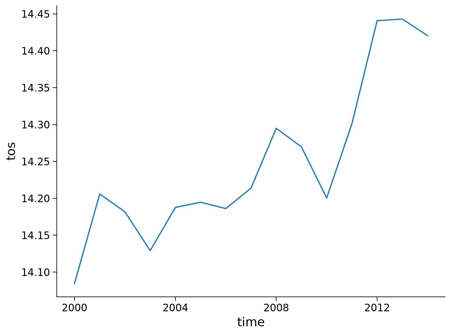
Our original SST data is monthly resolution. Let’s use .resample() to downsample to annual frequency:
# resample from a monthly to an annual frequency
tos_yearly = ds.tos.resample(time="AS")
tos_yearly
<string>:6: FutureWarning: 'AS' is deprecated and will be removed in a future version. Please use 'YS' instead of 'AS'.
DataArrayResample, grouped over '__resample_dim__'
15 groups with labels 2000-01-01, 00:00:00, ..., 201....
# calculate the global mean of the resampled data
annual_mean = tos_yearly.mean()
annual_mean_global = annual_mean.mean(dim=["lat", "lon"])
annual_mean_global.plot()
[<matplotlib.lines.Line2D at 0x7f732d7ad350>]
Section 1.2: Moving Average#
The .rolling() method allows for a rolling window aggregation and is applied along one dimension using the name of the dimension as a key (e.g. time) and the window size as the value (e.g. 6). We will use these values in the demonstration below.
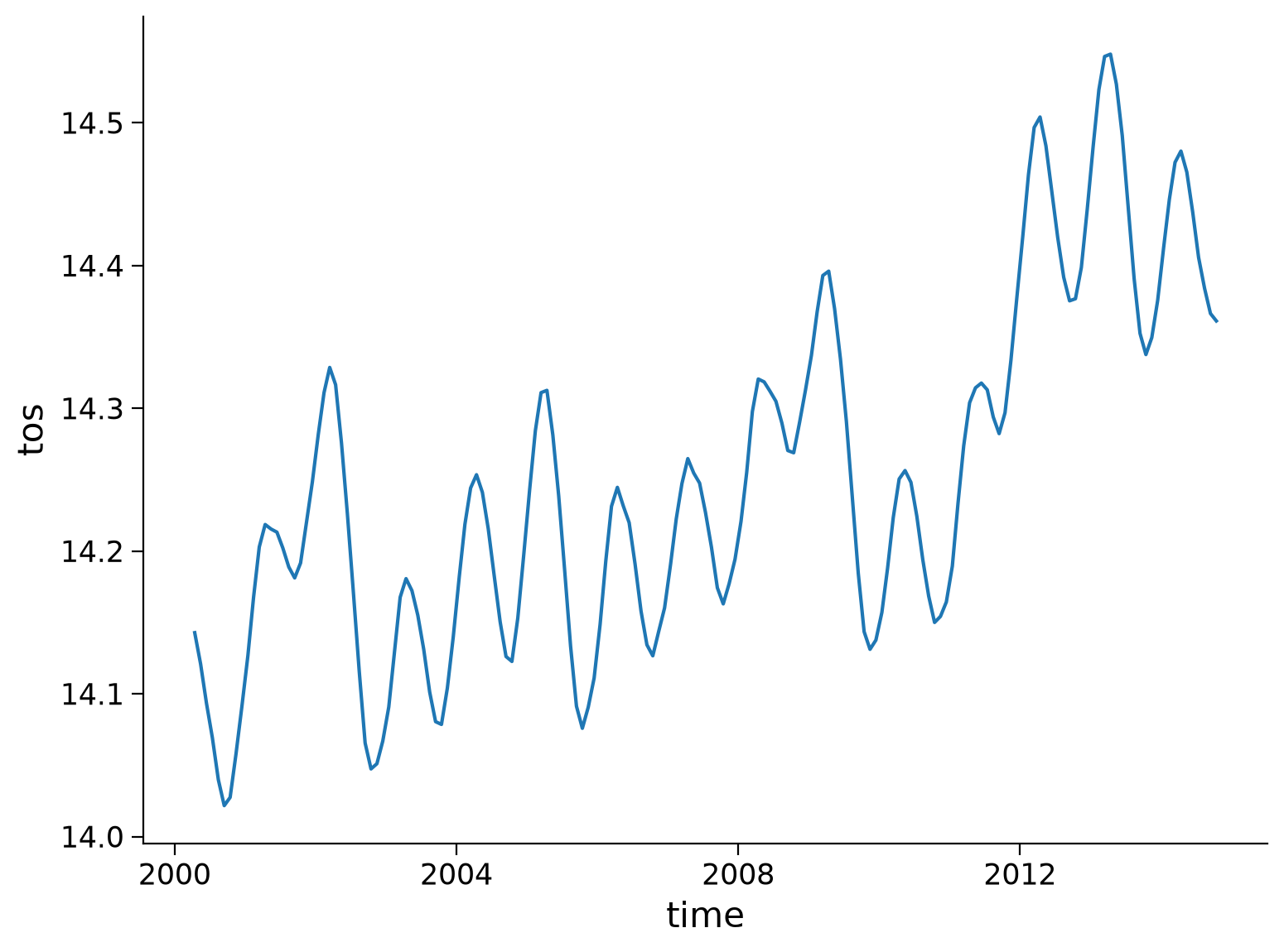
Let’s use the .rolling() function to compute a 6-month moving average of our SST data:
# calculate the running mean
tos_m_avg = ds.tos.rolling(time=6, center=True).mean()
tos_m_avg
<xarray.DataArray 'tos' (time: 180, lat: 180, lon: 360)> Size: 47MB
array([[[       nan,        nan,        nan, ...,        nan,
                nan,        nan],
        [       nan,        nan,        nan, ...,        nan,
                nan,        nan],
        [       nan,        nan,        nan, ...,        nan,
                nan,        nan],
        ...,
        [       nan,        nan,        nan, ...,        nan,
                nan,        nan],
        [       nan,        nan,        nan, ...,        nan,
                nan,        nan],
        [       nan,        nan,        nan, ...,        nan,
                nan,        nan]],

       [[       nan,        nan,        nan, ...,        nan,
                nan,        nan],
        [       nan,        nan,        nan, ...,        nan,
                nan,        nan],
        [       nan,        nan,        nan, ...,        nan,
                nan,        nan],
...
        [       nan,        nan,        nan, ...,        nan,
                nan,        nan],
        [       nan,        nan,        nan, ...,        nan,
                nan,        nan],
        [       nan,        nan,        nan, ...,        nan,
                nan,        nan]],

       [[       nan,        nan,        nan, ...,        nan,
                nan,        nan],
        [       nan,        nan,        nan, ...,        nan,
                nan,        nan],
        [       nan,        nan,        nan, ...,        nan,
                nan,        nan],
        ...,
        [       nan,        nan,        nan, ...,        nan,
                nan,        nan],
        [       nan,        nan,        nan, ...,        nan,
                nan,        nan],
        [       nan,        nan,        nan, ...,        nan,
                nan,        nan]]], dtype=float32)
Coordinates:
  * time     (time) object 1kB 2000-01-15 12:00:00 ... 2014-12-15 12:00:00
  * lat      (lat) float64 1kB -89.5 -88.5 -87.5 -86.5 ... 86.5 87.5 88.5 89.5
  * lon      (lon) float64 3kB 0.5 1.5 2.5 3.5 4.5 ... 356.5 357.5 358.5 359.5
Attributes: (12/19)
    cell_measures:  area: areacello
    cell_methods:   area: mean where sea time: mean
    comment:        Model data on the 1x1 grid includes values in all cells f...
    description:    This may differ from "surface temperature" in regions of ...
    frequency:      mon
    id:             tos
    ...             ...
    time_label:     time-mean
    time_title:     Temporal mean
    title:          Sea Surface Temperature
    type:           real
    units:          degC
variable_id: tos# calculate the global average of the running mean
tos_m_avg_global = tos_m_avg.mean(dim=["lat", "lon"])
tos_m_avg_global.plot()
[<matplotlib.lines.Line2D at 0x7f732d8fb990>]
Section 1.3: Coarsening the Data#
The .coarsen() function allows for block aggregation along multiple dimensions.
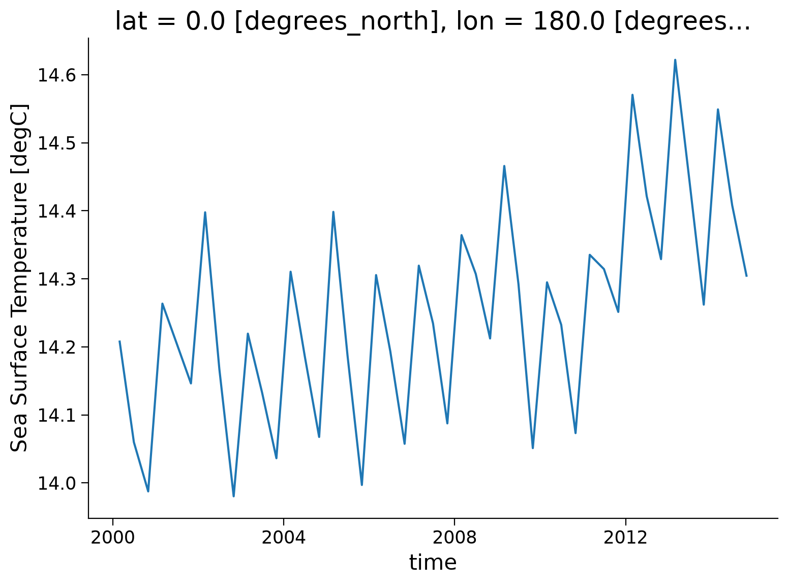
Let’s use the .coarsen() function to take a block mean for every 4 months and globally (i.e., 180 points along the latitude dimension and 360 points along the longitude dimension). Although we know the dimensions of our data quite well, we will include code that finds the length of the latitude and longitude variables so that it could work for other datasets that have a different format.
# coarsen the data
coarse_data = ds.coarsen(time=4, lat=len(ds.lat), lon=len(ds.lon)).mean()
coarse_data
<xarray.Dataset> Size: 1kB
Dimensions:    (time: 45, d2: 2, lat: 1, lon: 1)
Coordinates:
  * time       (time) object 360B 2000-03-01 00:00:00 ... 2014-10-30 18:00:00
  * lat        (lat) float64 8B 0.0
  * lon        (lon) float64 8B 180.0
Dimensions without coordinates: d2
Data variables:
    time_bnds  (time, d2) object 720B 2000-02-15 00:00:00 ... 2014-11-16 00:0...
    lat_bnds   (lat, d2) float64 16B -0.5 0.5
    lon_bnds   (lon, d2) float64 16B 179.5 180.5
    tos        (time, lat, lon) float32 180B 14.21 14.06 13.99 ... 14.41 14.3
Attributes: (12/45)
    Conventions:            CF-1.7 CMIP-6.2
    activity_id:            CMIP
    branch_method:          standard
    branch_time_in_child:   674885.0
    branch_time_in_parent:  219000.0
    case_id:                972
    ...                     ...
    sub_experiment_id:      none
    table_id:               Omon
    tracking_id:            hdl:21.14100/2975ffd3-1d7b-47e3-961a-33f212ea4eb2
    variable_id:            tos
    variant_info:           CMIP6 20th century experiments (1850-2014) with C...
variant_label: r11i1p1f1coarse_data.tos.plot()
[<matplotlib.lines.Line2D at 0x7f732a643290>]
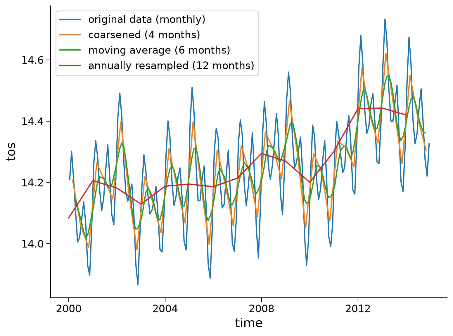
Section 1.4: Compare the Resampling Methods#
Now that we’ve tried multiple resampling methods on different temporal resolutions, we can compare the resampled datasets to the original.
original_global = ds.mean(dim=["lat", "lon"])
original_global.tos.plot(size=6)
coarse_data.tos.plot()
tos_m_avg_global.plot()
annual_mean_global.plot()


plt.legend(
    [
        "original data (monthly)",
        "coarsened (4 months)",
        "moving average (6 months)",
        "annually resampled (12 months)",
    ]
)
<matplotlib.legend.Legend at 0x7f732d81ae10>
Questions 1.4: Climate Connection#
What type of information can you obtain from each time series?
In what scenarios would you use different temporal resolutions?
Submit your feedback#
Show code cell source
# @title Submit your feedback
content_review(f"{feedback_prefix}_Questions_1_4")
Summary#
In this tutorial, we’ve explored Xarray tools to simplify and understand climate data better. Given the complexity and variability of climate data, tools like .resample(), .rolling(), and .coarsen() come in handy to make the data easier to compare and find long-term trends. You’ve also looked at valuable techniques like calculating moving averages.
Resources#
Code and data for this tutorial is based on existing content from Project Pythia.