Tutorial 2: Building and Training Random Forest Models

Tutorial 2: Building and Training Random Forest Models#

Week 2, Day 5, AI and Climate Change

Content creators: Deepak Mewada, Grace Lindsay

Content reviewers: Mujeeb Abdulfatai, Nkongho Ayuketang Arreyndip, Jeffrey N. A. Aryee, Paul Heubel, Jenna Pearson, Abel Shibu

Content editors: Deepak Mewada, Grace Lindsay

Production editors: Konstantine Tsafatinos

Our 2024 Sponsors: CMIP, NFDI4Earth

Tutorial Objectives#

Estimated timing of tutorial: 35 minutes

In this tutorial, you will

Learn about decision trees and hyperparameters
Learn about random forest models
Understand how regression models are evaluated (R\(^2\))
Familiarize yourself with the scikit-learn package

Setup#

# imports
import matplotlib.pyplot as plt                           # For plotting graphs
import pandas as pd                                       # For data manipulation
import ipywidgets as widgets                              # interactive display
from sklearn.ensemble import RandomForestRegressor        # For Random Forest Regression
from sklearn.tree import DecisionTreeRegressor            # For Decision Tree Regression
from sklearn.tree import plot_tree                        # For plotting decision trees

Figure Settings#

Set random seed#

Executing set_seed(seed=seed) you are setting the seed

Random seed 42 has been set.

Video 1: Building and training Random Forest Models#

Section 1: Preparing the Data for Model Training#

In this video, we learned about:

Using regression for prediction tasks, like the one we have.
The conceptual understanding of decision trees and their regression capabilities.
Random forests as an ensemble of decision trees.
Training our model
Measuring model performance.
Utilizing the scikit-learn toolbox for regression tasks.

Section 1.1: Loading the data#

Remember from the previous tutorial how we loaded the training_data? Let’s again load the data here for this tutorial.

#Load Dataset
url_Climatebench_train_val = "https://osf.io/y2pq7/download"
training_data = pd.read_csv(url_Climatebench_train_val)

Next, we will prepare the data to train a model to predict temperature anomalies in 2050. Let’s also remind ourselves of what the data contains:

Section 1.2: Preparing the data#

# Check column names (assuming a pandas DataFrame)
print("Column names:")
print(training_data.columns.tolist())  # List all column names

Column names:
['scenario', 'lat', 'lon', 'tas_2015', 'pr_2015', 'pr90_2015', 'dtr_2015', 'tas_FINAL', 'CO2_2015', 'SO2_2015', 'CH4_2015', 'BC_2015', 'CO2_2016', 'SO2_2016', 'CH4_2016', 'BC_2016', 'CO2_2017', 'SO2_2017', 'CH4_2017', 'BC_2017', 'CO2_2018', 'SO2_2018', 'CH4_2018', 'BC_2018', 'CO2_2019', 'SO2_2019', 'CH4_2019', 'BC_2019', 'CO2_2020', 'SO2_2020', 'CH4_2020', 'BC_2020', 'CO2_2021', 'SO2_2021', 'CH4_2021', 'BC_2021', 'CO2_2022', 'SO2_2022', 'CH4_2022', 'BC_2022', 'CO2_2023', 'SO2_2023', 'CH4_2023', 'BC_2023', 'CO2_2024', 'SO2_2024', 'CH4_2024', 'BC_2024', 'CO2_2025', 'SO2_2025', 'CH4_2025', 'BC_2025', 'CO2_2026', 'SO2_2026', 'CH4_2026', 'BC_2026', 'CO2_2027', 'SO2_2027', 'CH4_2027', 'BC_2027', 'CO2_2028', 'SO2_2028', 'CH4_2028', 'BC_2028', 'CO2_2029', 'SO2_2029', 'CH4_2029', 'BC_2029', 'CO2_2030', 'SO2_2030', 'CH4_2030', 'BC_2030', 'CO2_2031', 'SO2_2031', 'CH4_2031', 'BC_2031', 'CO2_2032', 'SO2_2032', 'CH4_2032', 'BC_2032', 'CO2_2033', 'SO2_2033', 'CH4_2033', 'BC_2033', 'CO2_2034', 'SO2_2034', 'CH4_2034', 'BC_2034', 'CO2_2035', 'SO2_2035', 'CH4_2035', 'BC_2035', 'CO2_2036', 'SO2_2036', 'CH4_2036', 'BC_2036', 'CO2_2037', 'SO2_2037', 'CH4_2037', 'BC_2037', 'CO2_2038', 'SO2_2038', 'CH4_2038', 'BC_2038', 'CO2_2039', 'SO2_2039', 'CH4_2039', 'BC_2039', 'CO2_2040', 'SO2_2040', 'CH4_2040', 'BC_2040', 'CO2_2041', 'SO2_2041', 'CH4_2041', 'BC_2041', 'CO2_2042', 'SO2_2042', 'CH4_2042', 'BC_2042', 'CO2_2043', 'SO2_2043', 'CH4_2043', 'BC_2043', 'CO2_2044', 'SO2_2044', 'CH4_2044', 'BC_2044', 'CO2_2045', 'SO2_2045', 'CH4_2045', 'BC_2045', 'CO2_2046', 'SO2_2046', 'CH4_2046', 'BC_2046', 'CO2_2047', 'SO2_2047', 'CH4_2047', 'BC_2047', 'CO2_2048', 'SO2_2048', 'CH4_2048', 'BC_2048', 'CO2_2049', 'SO2_2049', 'CH4_2049', 'BC_2049', 'CO2_2050', 'SO2_2050', 'CH4_2050', 'BC_2050']

First, we will drop the scenario column from the data as it is just a label, but will not be passed into the model.

training_data.pop('scenario')

             ssp126
             ssp126
             ssp126
             ssp126
             ssp126
             ...      
  ssp370-lowNTCF
  ssp370-lowNTCF
  ssp370-lowNTCF
  ssp370-lowNTCF
  ssp370-lowNTCF
Name: scenario, Length: 3240, dtype: object

As we can see, scenario is no longer in the dataset:

print("Column names:")
print(training_data.columns.tolist())  # List all column names

Column names:
['lat', 'lon', 'tas_2015', 'pr_2015', 'pr90_2015', 'dtr_2015', 'tas_FINAL', 'CO2_2015', 'SO2_2015', 'CH4_2015', 'BC_2015', 'CO2_2016', 'SO2_2016', 'CH4_2016', 'BC_2016', 'CO2_2017', 'SO2_2017', 'CH4_2017', 'BC_2017', 'CO2_2018', 'SO2_2018', 'CH4_2018', 'BC_2018', 'CO2_2019', 'SO2_2019', 'CH4_2019', 'BC_2019', 'CO2_2020', 'SO2_2020', 'CH4_2020', 'BC_2020', 'CO2_2021', 'SO2_2021', 'CH4_2021', 'BC_2021', 'CO2_2022', 'SO2_2022', 'CH4_2022', 'BC_2022', 'CO2_2023', 'SO2_2023', 'CH4_2023', 'BC_2023', 'CO2_2024', 'SO2_2024', 'CH4_2024', 'BC_2024', 'CO2_2025', 'SO2_2025', 'CH4_2025', 'BC_2025', 'CO2_2026', 'SO2_2026', 'CH4_2026', 'BC_2026', 'CO2_2027', 'SO2_2027', 'CH4_2027', 'BC_2027', 'CO2_2028', 'SO2_2028', 'CH4_2028', 'BC_2028', 'CO2_2029', 'SO2_2029', 'CH4_2029', 'BC_2029', 'CO2_2030', 'SO2_2030', 'CH4_2030', 'BC_2030', 'CO2_2031', 'SO2_2031', 'CH4_2031', 'BC_2031', 'CO2_2032', 'SO2_2032', 'CH4_2032', 'BC_2032', 'CO2_2033', 'SO2_2033', 'CH4_2033', 'BC_2033', 'CO2_2034', 'SO2_2034', 'CH4_2034', 'BC_2034', 'CO2_2035', 'SO2_2035', 'CH4_2035', 'BC_2035', 'CO2_2036', 'SO2_2036', 'CH4_2036', 'BC_2036', 'CO2_2037', 'SO2_2037', 'CH4_2037', 'BC_2037', 'CO2_2038', 'SO2_2038', 'CH4_2038', 'BC_2038', 'CO2_2039', 'SO2_2039', 'CH4_2039', 'BC_2039', 'CO2_2040', 'SO2_2040', 'CH4_2040', 'BC_2040', 'CO2_2041', 'SO2_2041', 'CH4_2041', 'BC_2041', 'CO2_2042', 'SO2_2042', 'CH4_2042', 'BC_2042', 'CO2_2043', 'SO2_2043', 'CH4_2043', 'BC_2043', 'CO2_2044', 'SO2_2044', 'CH4_2044', 'BC_2044', 'CO2_2045', 'SO2_2045', 'CH4_2045', 'BC_2045', 'CO2_2046', 'SO2_2046', 'CH4_2046', 'BC_2046', 'CO2_2047', 'SO2_2047', 'CH4_2047', 'BC_2047', 'CO2_2048', 'SO2_2048', 'CH4_2048', 'BC_2048', 'CO2_2049', 'SO2_2049', 'CH4_2049', 'BC_2049', 'CO2_2050', 'SO2_2050', 'CH4_2050', 'BC_2050']

Next, we need to pull out our target variable (that is, the variable we want our model to predict). Here that is tas_FINAL, the temperature anomaly in 2050. The anomalies in every case are calculated by subtracting the annual means of the pre-industrial scenario from the annual means of the respective scenario of interest.

target = training_data.pop('tas_FINAL')
target

     0.848419
     0.737915
     0.588806
     0.522766
     0.776642
          ...   
  1.626139
  1.804036
  1.925557
  2.026601
  2.162618
Name: tas_FINAL, Length: 3240, dtype: float64

Note: we will need to repeat these preprocessing steps anytime we load this (or other) data.

Section 2: Fit Decision Tree and Random Forest#

Now we can train our models. As mentioned in the video, Decision Trees and Random Forest Models can both do regression. Specifically:

Decision Tree Regression:

Decision trees recursively partition the feature space into regions based on feature values to predict the target variable.
Each leaf node represents a prediction.
Single trees can be prone to capturing noise in the data (not what we want!).

Random Forest Regression:

An ensemble method that combines multiple decision trees to improve predictive performance.
Each tree is trained on a random subset of the data.
Aggregates predictions of individual trees to improve performance.
Typically more robust/doesn’t capture noise.

We will see an example of both here.

First, let’s train a single decision tree to try to predict 2050 temperature anomalies using 2015 temperature anomalies and emissions data. We can control the depth of our decision tree (which is the maximum number of splits performed), which we will set to 20 here.

Section 2.0: Scikit-learn#

In this and coming sub-sections, we will utilize Scikit-learn, commonly referred to as sklearn, a renowned Python library extensively employed for machine learning endeavors. It provides a comprehensive array of functions and tools tailored for various machine learning tasks. Specifically, we will concentrate on the DecisionTreeRegressor and RandomForestRegressor modules offered by Scikit-learn.

Section 2.1: Training the Decision Tree and Analyzing the Results#

# instantiate the model:
dt_regressor = DecisionTreeRegressor(random_state=random_state,max_depth=20)

# fit/train the model with the data:
dt_regressor.fit(training_data, target) #pass in the model inputs and the target it should predict

DecisionTreeRegressor(max_depth=20, random_state=42)

In a Jupyter environment, please rerun this cell to show the HTML representation or trust the notebook.
On GitHub, the HTML representation is unable to render, please try loading this page with nbviewer.org.

We’ve trained our first model! Now let’s see how well it performs. As discussed in the video, we will use the coefficient of determination (also known as the R-squared value, \(R^2\)) as the measure of how well the model is doing.

We can get this value by calling the score function and providing the data we want the score calculated on. Here we will evaluate the model on the same data it was trained on.

Learn more about the R-Squared value and Coefficient of determination

The R-squared value indicates the proportion of the variance in the target variable that is predicted from the model.

Specifically, the coefficient of determination is calculated using the formula:

\[ \color{#3182CE}{R^2} = 1 - \frac{\color{#DC3912}{SS_{\text{residual}}}}{\color{#FF9900}{SS_{\text{total}}}} \]

where:

\(\color{#FF9900}{SS_{\text{total}}}\) represents the total sum of squares, calculated as the sum of squared differences between the target variable \(\color{#2CA02C}{y}\) and its mean \(\color{#2CA02C}{\bar{y}}\):

\[ \color{#FF9900}{SS_{\text{total}}} = \sum_{i=1}^{n} (\color{#2CA02C}{y_i} - \color{#2CA02C}{\bar{y}})^2 \]

\(\color{#DC3912}{SS_{\text{residual}}}\) denotes the residual sum of squares, computed as the sum of squared differences between the observed target values \(\color{#2CA02C}{y}\) and the predicted values \(\color{#FF5733}{\hat{y}}\) provided by the model:

\[ \color{#DC3912}{SS_{\text{residual}}} = \sum_{i=1}^{n} (\color{#2CA02C}{y_i} - \color{#FF5733}{\hat{y}_i})^2 \]

The \(\color{#3182CE}{R^2}\) score thus quantifies the proportion of variance in the target variable that is predictable from the independent variables in the model.

This value ranges from 0 to 1, where 1 indicates a perfect fit, meaning the model explains all the variability in the target variable.

dt_regressor.score(training_data, target)

0.9983600129961374

Now, let’s create a scatter plot to compare the true temperature anomaly values in 2050 to those predicted by the model:

Scatter Plot: Predicted vs. True Temperatures for Decision Tree#

../../../_images/288a424c457198b3d16f7e0e1a999e82177fbda76f9b2070e28c29f270c381f8.png

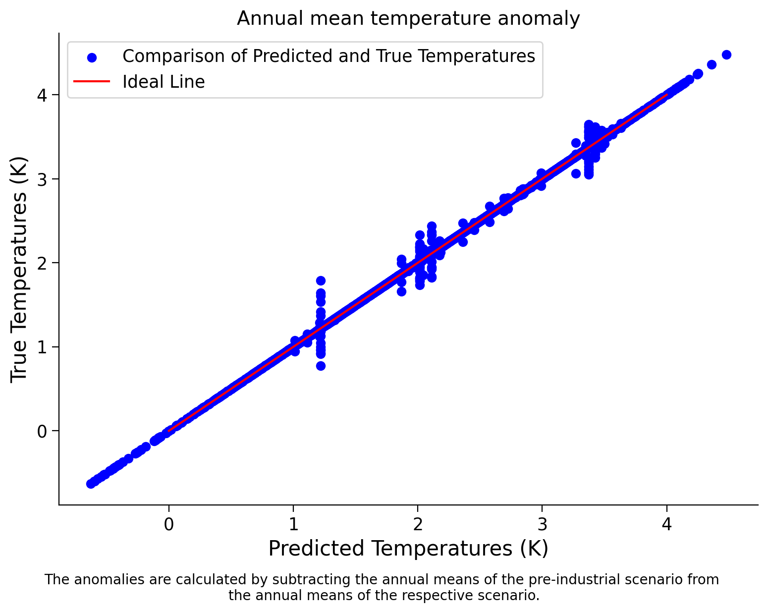
What can we conclude from this score and the scatter plot?
First, pause and think by yourself. Then, compare it with the information provided here:

As we can see, the model achieves a high score of ~0.9984 on the training data. This indicates that the model can explain approximately 99.84% of the variance in the target variable based on the features in the training dataset. Such a high score suggests that the model fits the training data very well and can effectively capture the underlying patterns or relationships between the features and the target variable. We can see the close alignment between the true value and the value predicted by the model in the plot.

However, it’s essential to note that achieving a high score on the training data does not guarantee the model’s performance on unseen data (i.e., the test or validation datasets). We will explore this more in the next tutorial.

Interactive Demo 2.1: Variation in Performance with depth | Visualizing Decision Trees and Scatter plot#

In this interactive demo, we’ll visualize decision trees using a widget. This widget enables interactive exploration of decision trees by adjusting two parameters:
max_depth controls the tree’s complexity during training, while dt_vis_depth determines the depth of the tree to visualize. It dynamically trains a decision tree regressor based on max_depth, evaluates its performance with a scatter plot, and visualizes the tree structure up to dt_vis_depth using the plot_tree function.
This allows users to balance model complexity and interpretability, gaining insights into how different depths affect predictive accuracy and tree structure.

Make sure you execute this cell to enable the widget!

Show code cell source Hide code cell source

# @markdown Make sure you execute this cell to enable the widget!
# Don't worry about understanding this code! It's to set up an interactive plot.

# Function to train decision tree and display scatter plot
def train_and_plot(max_depth, visualize_depth):
    global dt_regressor, training_data

    # Instantiate and train the decision tree regressor
    dt_regressor = DecisionTreeRegressor(max_depth=max_depth)
    dt_regressor.fit(training_data, target)

    # Calculate and print the score
    score = dt_regressor.score(training_data, target)
    print(f"Model Score: {score}")
    print(f"Please wait for ~{visualize_depth+visualize_depth/2} sec for the figure to render")
    # Generate scatter plot: Predicted vs. True Temperatures
    predicted = dt_regressor.predict(training_data)
    fig, axes = plt.subplots(1, 2, figsize=(15+pow(1.3,visualize_depth), 6+pow(1.2,visualize_depth)), gridspec_kw={'width_ratios': [1, 1+visualize_depth/4]})

    # Scatter plot
    axes[0].scatter(predicted, target, color='blue', alpha=0.7, label='Comparison of Predicted and True Temperatures', edgecolors='black')
    axes[0].plot([min(target), max(target)], [min(target), max(target)], color='red', linestyle='--', label='Ideal Prediction Line')
    axes[0].set_xlabel('Predicted Temperature (K)', fontsize=12)
    axes[0].set_ylabel('True Temperature (K)', fontsize=12)
    axes[0].set_title('Annual mean temperature anomaly', fontsize=14)
    axes[0].legend()
    axes[0].grid(True)

    # Decision tree visualization
    plot_tree(dt_regressor, feature_names=training_data.columns, filled=True, fontsize=8, max_depth=visualize_depth, ax=axes[1])
    axes[1].set_title(f'Decision Tree Visualization (Train_max_depth = {max_depth}, dt_visualize_depth = {visualize_depth})')

    plt.tight_layout()
    plt.show()

# Interactive widget to control max_depth
@widgets.interact(max_depth=(1, 31, 1), dt_vis_depth=(1, 10, 1))
def visualize_tree_with_max_depth(max_depth=20, dt_vis_depth=3):
    train_and_plot(max_depth, dt_vis_depth)

Interactive Demo 2.1 Discussion#

How does changing the max_depth parameter affect the decision tree’s predictive accuracy and complexity?
What insights can be gained by visualizing the decision tree at different depths (dt_vis_depth)?
What patterns or trends do you observe in the residuals (differences between predicted and true temperatures) on the scatter plot? How can these insights guide adjustments to improve the model’s predictive accuracy?

Click for solution

Section 2.2: Training the Random forest and Analyzing the Results#

Now we will train an ensemble of decisions trees, known as a random forest. For this we can use the built-in RandomForestRegressor from the sklearn.ensemble.RandomForestRegressor, which we have already imported.

rf_regressor = RandomForestRegressor(random_state=random_state)

The line of code creates a random forest regressor object named rf_regressor. This regressor is configured to use a specified random_state parameter, ensuring that the random number generation process within the algorithm is consistent across different runs. This helps maintain reproducibility in our experiments and ensures consistent results.

Now you will train the model on our data and calculate its score on the same data. Create a plot like the one above in order to visually inspect its performance

Coding Exercise 2.2: Model Training and Performance Visualization of Ranodm Forest#

In this exercise, you will train a random forest regressor model on your data and evaluate its performance by calculating its score on the same data. Additionally, you will create a scatter plot to visually inspect its performance.

def fit_and_visualize_rf(training_data, target):
    """Fit a random forest regressor to the training data and visualize the results.

    Args:
        training_data (array-like): Input data for training the model.
        target (array-like): Target variable for training the model.

    Returns:
        None
    """
    #################################################
    ## TODO for students: Fit the random forest regressor and visualize the results ##
    # Remove the following line of code once you have completed the exercise:
    raise NotImplementedError("Student exercise: Fit the random forest regressor and visualize the results.")
    #################################################

    # fit the random forest regressor to the training data
    _ = ...

    # print the R-squared score of the model
    print('...')

    # predict the target variable using the trained model
    predicted = rf_regressor.predict(training_data)

    # Create scatter plot
    plt.scatter(predicted,target,color='b',label='Comparison of Predicted and True Temperatures')
    plt.plot([0,4],[0,4],color='r', label='Ideal Line') # add a diagonal line for reference
    plt.xlabel('Predicted Temperatures (K)')
    plt.ylabel('True Temperatures (K)')
    plt.legend()
    plt.title('Annual mean temperature anomaly')
    # add a caption with adjusted y-coordinate to create space
    caption_text = 'The anomalies are calculated by subtracting the annual means of the pre-industrial scenario from \nthe annual means of the respective scenario.'
    plt.figtext(0.5, -0.03, caption_text, ha='center', fontsize=10)  # adjusted y-coordinate to create space

# test your function
_ = fit_and_visualize_rf(training_data, target)

Click for solution

Example output:

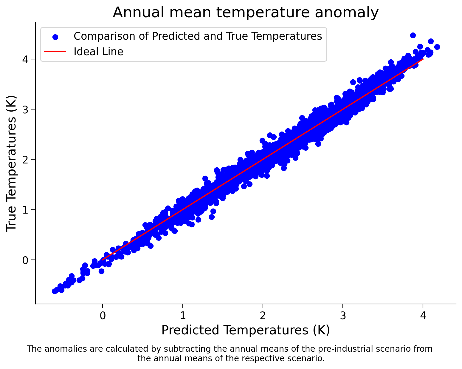
It seems like our models are performing very well! Let’s think a bit more in the next tutorial about what else we should do to evaluate our models…

Summary#

Estimated timing of tutorial: 35 minutes

In this tutorial, we delved into Random Forest Models and their application in climate prediction. We gained an understanding of regression and how Random Forests combine decision trees to improve predictive accuracy. Through practical exercises, we learned how to evaluate model performance and implement Random Forests using tools like scikit-learn.

Resources#

ClimateBench v1.0: A Benchmark for Data-Driven Climate Projections

Tutorial 2: Building and Training Random Forest Models

Contents

Tutorial 2: Building and Training Random Forest Models#

Tutorial Objectives#

Setup#

Figure Settings#

Set random seed#

Video 1: Building and training Random Forest Models#

Section 1: Preparing the Data for Model Training#

Section 1.1: Loading the data#

Section 1.2: Preparing the data#

Section 2: Fit Decision Tree and Random Forest#

Section 2.0: Scikit-learn#

Section 2.1: Training the Decision Tree and Analyzing the Results#

Scatter Plot: Predicted vs. True Temperatures for Decision Tree#

Interactive Demo 2.1: Variation in Performance with depth | Visualizing Decision Trees and Scatter plot#

Interactive Demo 2.1 Discussion#

Section 2.2: Training the Random forest and Analyzing the Results#

Coding Exercise 2.2: Model Training and Performance Visualization of Ranodm Forest#

Summary#

Resources#