![]()

Tutorial 5: Paleoclimate Data Analysis Tools#
Week 1, Day 4, Paleoclimate
Content creators: Sloane Garelick
Content reviewers: Yosmely Bermúdez, Dionessa Biton, Katrina Dobson, Maria Gonzalez, Will Gregory, Nahid Hasan, Paul Heubel, Sherry Mi, Beatriz Cosenza Muralles, Brodie Pearson, Jenna Pearson, Chi Zhang, Ohad Zivan
Content editors: Yosmely Bermúdez, Paul Heubel, Zahra Khodakaramimaghsoud, Jenna Pearson, Agustina Pesce, Chi Zhang, Ohad Zivan
Production editors: Wesley Banfield, Paul Heubel, Jenna Pearson, Konstantine Tsafatinos, Chi Zhang, Ohad Zivan
Our 2024 Sponsors: CMIP, NFDI4Earth
Tutorial Objectives#
Estimated timing of tutorial: 30 minutes
In this tutorial, you will explore various computational analyses for interpreting paleoclimate data and understand why these methods are useful. A common issue in paleoclimate is the presence of uneven time spacing between consecutive observations. Pyleoclim includes several methods that can deal with uneven sampling effectively, but there are certain applications and analyses for which it’s necessary to place the records on a uniform time axis. In this tutorial, you’ll learn a few ways to do this with Pyleoclim. Additionally, we will explore another useful paleoclimate data analysis tool, Principal Component Analysis (PCA), which allows us to identify a common signal between various paleoclimate reconstructions.
By the end of this tutorial, you’ll be able to perform the following data analysis techniques on proxy-based climate reconstructions:
Interpolation
Binning
Principal component analysis (PCA)
Setup#
# installations ( uncomment and run this cell ONLY when using google colab or kaggle )

# !pip install pyleoclim
# imports

# for Google Colab users: you might get a numpy.dtype error here, restart your session and rerun the code and it should solve it.
import pandas as pd
import pyleoclim as pyleo
import matplotlib.pyplot as plt
import pooch
import os
import tempfile

from sklearn.decomposition import PCA
Install and import feedback gadget#
Show code cell source
# @title Install and import feedback gadget

!pip3 install vibecheck datatops --quiet

from vibecheck import DatatopsContentReviewContainer
def content_review(notebook_section: str):
    return DatatopsContentReviewContainer(
        "",  # No text prompt
        notebook_section,
        {
            "url": "https://pmyvdlilci.execute-api.us-east-1.amazonaws.com/klab",
            "name": "comptools_4clim",
            "user_key": "l5jpxuee",
        },
    ).render()


feedback_prefix = "W1D4_T5"
Figure Settings#
Show code cell source
# @title Figure Settings
import ipywidgets as widgets  # interactive display

%config InlineBackend.figure_format = 'retina'
plt.style.use(
    "https://raw.githubusercontent.com/neuromatch/climate-course-content/main/cma.mplstyle"
)
Helper functions#
Show code cell source
# @title Helper functions

def pooch_load(filelocation=None, filename=None, processor=None):
    shared_location = "/home/jovyan/shared/Data/tutorials/W1D4_Paleoclimate"  # this is different for each day
    user_temp_cache = tempfile.gettempdir()

    if os.path.exists(os.path.join(shared_location, filename)):
        file = os.path.join(shared_location, filename)
    else:
        file = pooch.retrieve(
            filelocation,
            known_hash=None,
            fname=os.path.join(user_temp_cache, filename),
            processor=processor,
        )

    return file
Video 1: Proxy Data Analysis Tools#
Submit your feedback#
Show code cell source
# @title Submit your feedback
content_review(f"{feedback_prefix}_Proxy_Data_Analysis_Tools_Video")
If you want to download the slides: https://osf.io/download/ujbqz/
Submit your feedback#
Show code cell source
# @title Submit your feedback
content_review(f"{feedback_prefix}_Proxy_Data_Analysis_Tools_Slides")
Section 1: Load the sample dataset for analysis#
For this tutorial, we are going to use an example dataset to practice the various data analysis techniques. The dataset we’ll be using is a record of hydrogen isotopes of leaf waxes (δDwax) from Lake Tanganyika in East Africa (Tierney et al., 2008). Recall from the video that δDwax is a proxy that is typically thought to record changes in the amount of precipitation in the tropics via the amount effect. In the previous tutorial, we looked at δD data from high-latitude ice cores. In that case, δD was a proxy for temperature, but in the tropics, δD more commonly reflects rainfall amount, as explained in the introductory video.
Let’s first read the data from a .csv file.
filename_tang = "tanganyika_dD.csv"
url_tang = "https://osf.io/sujvp/download/"
tang_dD = pd.read_csv(pooch_load(filelocation=url_tang, filename=filename_tang))
tang_dD.head()
Downloading data from 'https://osf.io/sujvp/download/' to file '/tmp/tanganyika_dD.csv'.
SHA256 hash of downloaded file: 66ef1d84b66cf5f78dc95d41e64a854af30508d49514c82cad266606be7b8345
Use this value as the 'known_hash' argument of 'pooch.retrieve' to ensure that the file hasn't changed if it is downloaded again in the future.
| Age | dD | dD_IVbio | dD_IVonly | d13C | |
|---|---|---|---|---|---|
| 0 | 1405 | -105.2 | -15.6 | -105.1 | -31.4 |
| 1 | 1769 | -97.3 | -6.9 | -97.2 | -30.7 |
| 2 | 1997 | -93.7 | -2.8 | -93.5 | -30.4 |
| 3 | 2316 | -107.8 | -18.5 | -107.8 | -29.8 |
| 4 | 2545 | -103.1 | -13.5 | -103.2 | -30.4 |
We can now create a Series in Pyleoclim and assign names to different variables so that we can easily plot the data.
ts_tang = pyleo.Series(
    time=tang_dD["Age"],
    value=tang_dD["dD_IVonly"],
    time_name="Age",
    time_unit="yr BP",
    value_name="dDwax",
    value_unit="per mille",
    label="Lake Tanganyika dDprecip",
)

ts_tang.plot(color="C1", invert_yaxis=True)
Time axis values sorted in ascending order
(<Figure size 1000x400 with 1 Axes>,
 <Axes: xlabel='Age [yr BP]', ylabel='dDwax [per mille]'>)
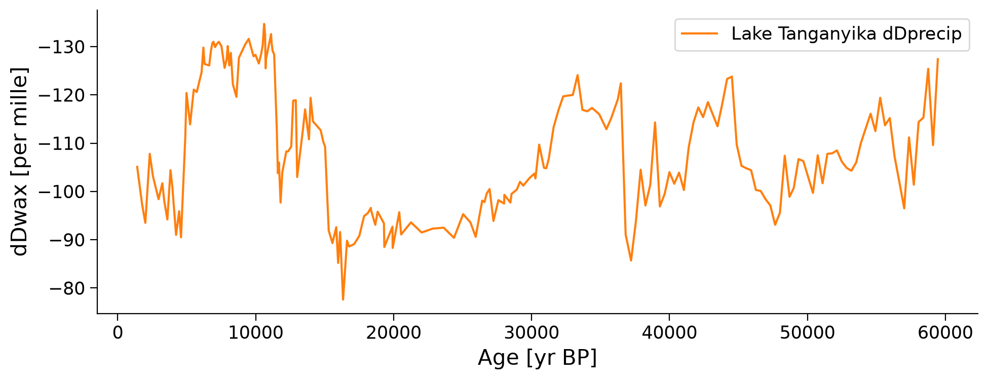
You may notice that the y-axis is inverted. When we’re plotting δD data, we typically invert the y-axis because more negative (“depleted”) values suggest increased rainfall, whereas more positive (“enriched”) values suggest decreased rainfall.
Section 2: Uniform Time-Sampling of the Data#
There are a number of different reasons we might want to assign new values to our data. For example, if the data is not evenly spaced, we might need to resample in order to use a sepcific data analysis technique or to more easily compare to other data of a different sampling resolution.
First, let’s check whether our data is already evenly spaced using the .is_evenly_spaced() method:
ts_tang.is_evenly_spaced()
False
Our data is not evenly spaced. There are a few different methods available in pyleoclim to place the data on a uniform axis, and in this tutorial, we’ll explore two methods: interpolating and binning. In general, these methods use the available data near a chosen time to estimate what the value was at that time, but each method differs in which nearby data points it uses and how it uses them.
Section 2.1: Interpolation#
To start out, let’s try using interpolation to evenly space our data. Interpolation projects the data onto an evenly spaced time axis with a distance between points (step size) of our choosing. There are a variety of different methods by which the data can be interpolated, these being: linear, nearest, zero, slinear, quadratic, cubic, previous, and next. More on these and their associated key word arguments can be found in the documentation. By default, the function .interp() implements linear interpolation:
tang_linear = ts_tang.interp() # default method = 'linear'
# check whether or not the series is now evenly spaced
tang_linear.is_evenly_spaced()
True
Now that we’ve interpolated our data, let’s compare the original dataset to the linearly interpolated dataset we just created.
fig, ax = plt.subplots()  # assign a new plot axis
ts_tang.plot(ax=ax, label="Original", invert_yaxis=True)
tang_linear.plot(ax=ax, label="Linear")
<Axes: xlabel='Age [yr BP]', ylabel='dDwax [per mille]'>
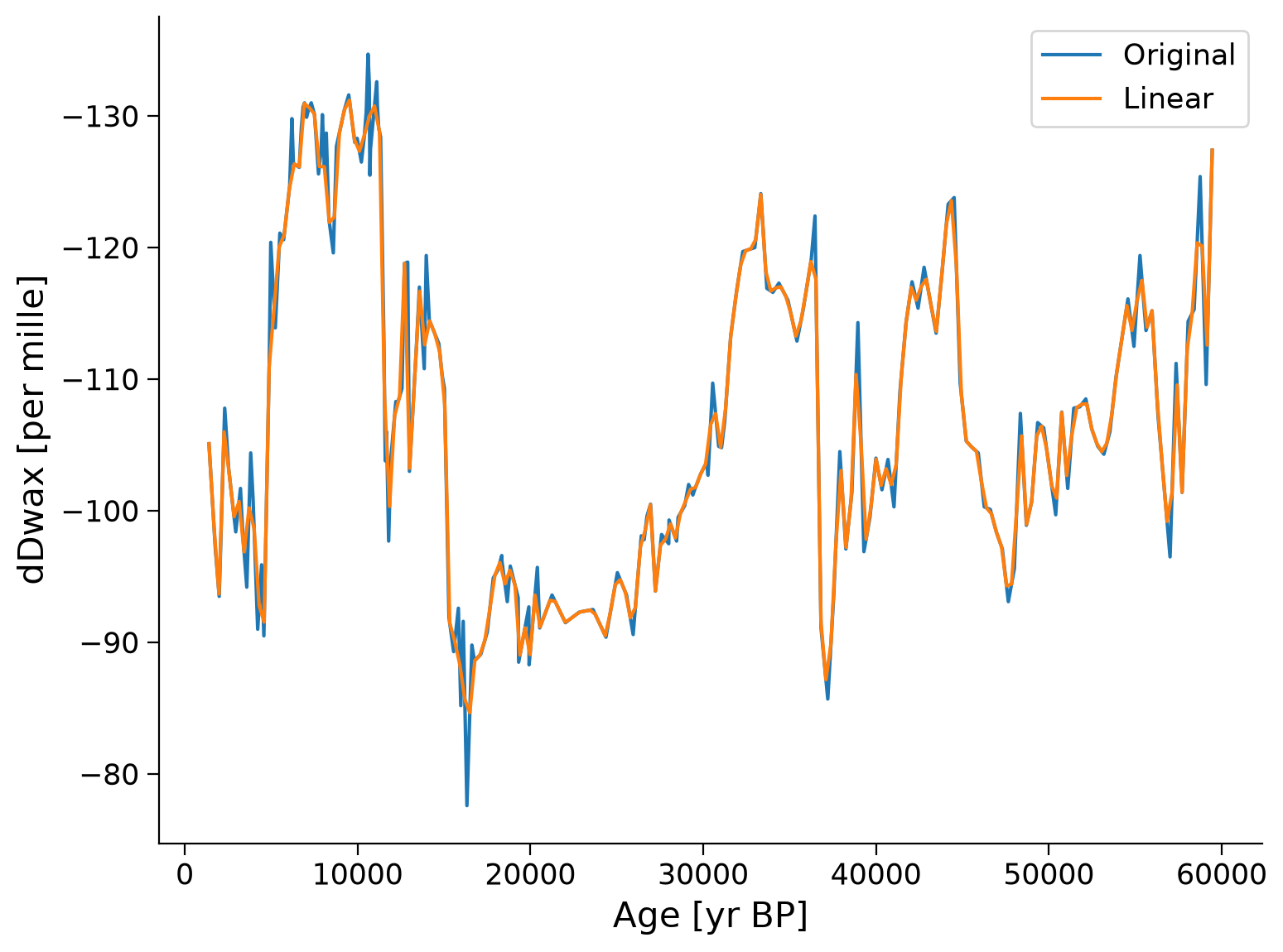
Notice there are only some minor differences between the original and linearly interpolated data.
You can print the data in the original and interpolated time series to see the difference in the ages between the two datasets. The interpolated dataset is now evenly spaced with a δD value every ~290 years.
ts_tang
{'label': 'Lake Tanganyika dDprecip'}
None
Age [yr BP]
1405.0    -105.1
1769.0     -97.2
1997.0     -93.5
2316.0    -107.8
2545.0    -103.2
           ...
58061.0   -114.4
58409.0   -115.3
58757.0   -125.4
59105.0   -109.6
59454.0   -127.4
Name: dDwax [per mille], Length: 201, dtype: float64
tang_linear
{'label': 'Lake Tanganyika dDprecip'}
None
Age [yr BP]
1405.000    -105.100000
1695.245     -98.800727
1985.490     -93.686785
2275.735    -105.995017
2565.980    -102.954380
                ...
58293.020   -115.000052
58583.265   -120.357691
58873.510   -120.110178
59163.755   -112.596673
59454.000   -127.400000
Name: dDwax [per mille], Length: 201, dtype: float64
Let’s compare a few of the different interpolation methods (e.g., quadratic, next, zero) with one another just to see how they are similar and different:
fig, ax = plt.subplots()  # assign a new plot axis
ts_tang.plot(ax=ax, label="original", invert_yaxis=True)
for method in ["linear", "quadratic", "next", "zero"]:
    ts_tang.interp(method=method).plot(
        ax=ax, label=method, alpha=0.9
    )  # plot all the method we want
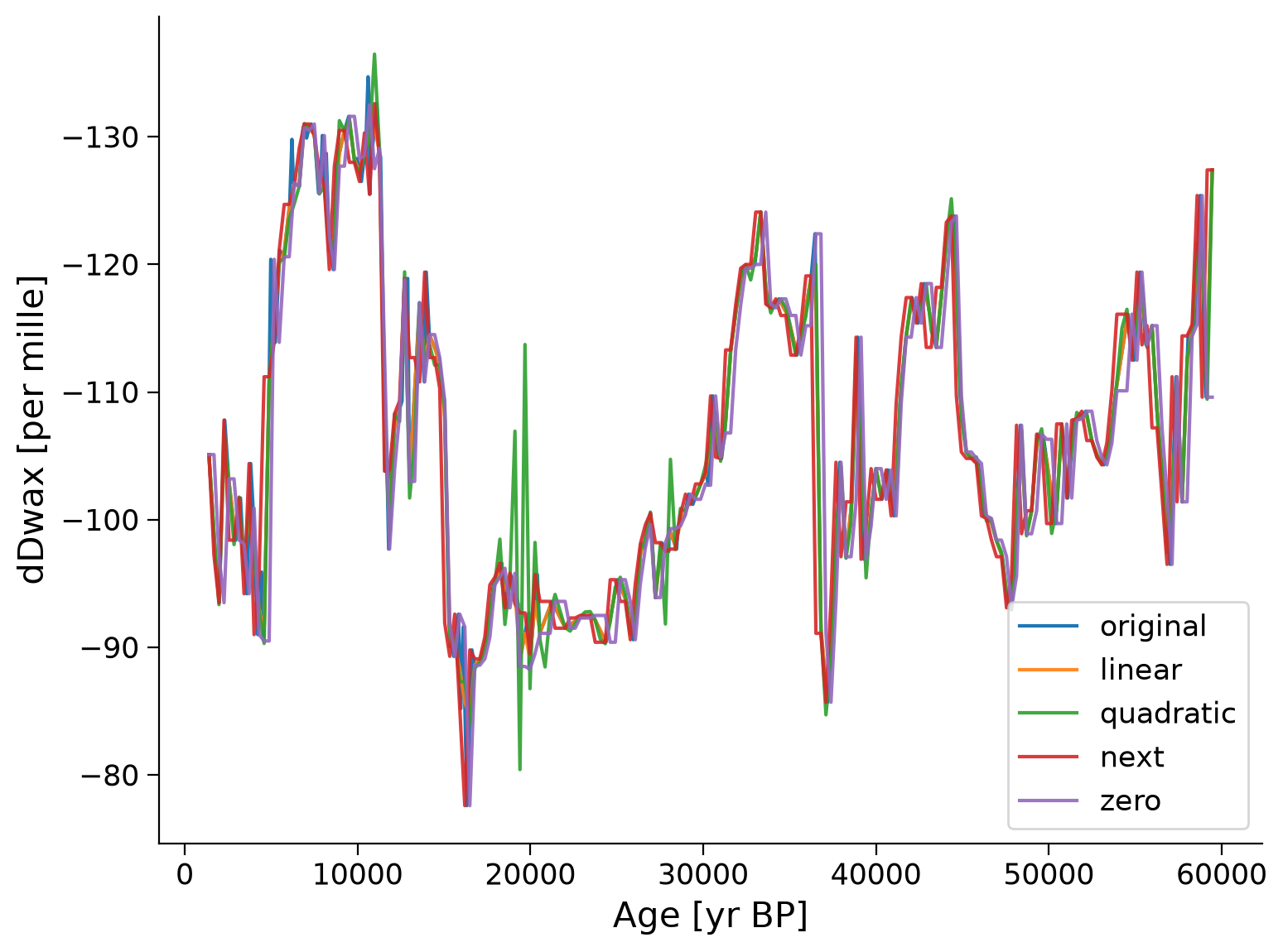
The methods can produce slightly different results, but mostly reproduce the same overall trend. In this case, the quadractic method may be less appropriate than the other methods.
Section 2.2: Binning#
Another option for resampling our data onto a uniform time axis is binning. Binning is when a set of time intervals is defined and data is grouped or binned with other data in the same interval, then all those points in a bin are averaged to get a data value for that bin. The defaults for binning pick a bin size at the coarsest time spacing present in the dataset and average data over a uniform sequence of such intervals.
tang_bin = (
    ts_tang.bin()
)  # default settings pick the coarsest time spacing in the data as the binning period
fig, ax = plt.subplots()  # assign a new plot axis
ts_tang.plot(ax=ax, label="Original", invert_yaxis=True)
tang_bin.plot(ax=ax, label="Binned")
<Axes: xlabel='Age [yr BP]', ylabel='dDwax [per mille]'>
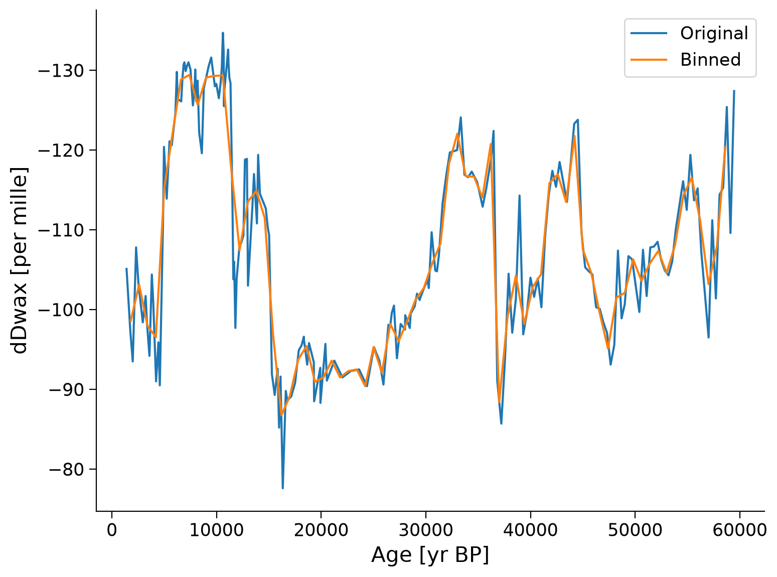
Again, notice that although there are some minor differences between the original and binned data, the records still capture the same overall trend.
Coding Exercises 2.2#
Experiment with different bin sizes to see how this affects the resampling. You can do so by adding
bin_size =tots_tang.bin(). Try a bin size of 500 years and 1,000 years and plot both of them on the same graph as the original data and the binned data using the default bin size.
# bin size of 500
tang_bin_500 = ...

# bin size of 1000
tang_bin_1000 = ...

# plot
fig, ax = plt.subplots()  # assign a new plot axis
_ = ...
_ = ...
_ = ...
_ = ...
Example output:

Submit your feedback#
Show code cell source
# @title Submit your feedback
content_review(f"{feedback_prefix}_Coding_Exercises_2_2")
Section 3: Principal Component Analysis (PCA)#
Large datasets, such as global climate datasets, are often difficult to interpret due to their multiple dimensions. Although tools such as Xarray help us to organize large, multidimensional climate datasets, it can still sometimes be difficult to interpret certain aspects of such data. Principal Component Analysis (PCA) is a tool for reducing the dimensionality of such datasets and increasing interpretability with minimal modification or loss of data. In other words, PCA allows us to reduce the number of variables of a dataset while preserving as much information as possible.
The first step in PCA is to calculate a matrix that summarizes how the variables in a dataset all relate to one another. This matrix is then broken down into new uncorrelated variables that are linear combinations or mixtures of the initial variables. These new variables are the principal components. The initial dimensions of the dataset determine the number of principal components calculated. Most of the information within the initial variables is compressed into the first components. Additional details about PCA and the calculations involved can be found here or here.
Applied to paleoclimate, PCA can reduce the dimensionality of large paleoclimate datasets with multiple variables and can help us identify a common signal between various paleoclimate reconstructions. An example of a study that applies PCA to paleoclimate is Otto-Bliesner et al., 2014. This study applies PCA to rainfall reconstructions from models and proxies from throughout Africa to determine common climate signals in these reconstructions.
In this section, we will calculate the PCA of four δD paleoclimate records from Africa to assess common climate signals in the four records. In order to calculate the PCA of multiple paleoclimate time series, all of the records need to be on a common time step. To do so, we can apply the resampling tools we’ve learned in this tutorial.
So far, we’ve been looking at δD data from Lake Tanganyika in tropical East Africa. Let’s compare this δD record to other existing δD records from lake and marine sediment cores in tropical Africa from the Gulf of Aden (Tierney and deMenocal, 2017), Lake Bosumtwi (Shanahan et al., 2015), and the West African Margin (Tierney et al., 2017).
First, let’s load these datasets:
# Gulf of Aden
filename_aden = "aden_dD.csv"
url_aden = "https://osf.io/gm2v9/download/"
aden_dD = pd.read_csv(pooch_load(filelocation=url_aden, filename=filename_aden))
aden_dD.head()
Downloading data from 'https://osf.io/gm2v9/download/' to file '/tmp/aden_dD.csv'.
SHA256 hash of downloaded file: e76d8f6c216cd8afccadef525fd82c7e1ab11356b12a1add5b69dee4b803f2a2
Use this value as the 'known_hash' argument of 'pooch.retrieve' to ensure that the file hasn't changed if it is downloaded again in the future.
| depth_cm | age_calBP95- | age_calBP | age_calBP95+ | dDwax | dDwaxIVcorr | |
|---|---|---|---|---|---|---|
| 0 | 1.25 | -21 | 0 | 23 | -128.9 | -128.9 |
| 1 | 7.50 | 105 | 138 | 170 | -128.3 | -128.3 |
| 2 | 11.50 | 183 | 226 | 265 | -133.6 | -133.6 |
| 3 | 16.50 | 279 | 335 | 383 | -133.6 | -133.6 |
| 4 | 21.50 | 376 | 442 | 500 | -138.1 | -138.1 |
# Lake Bosumtwi
filename_Bosumtwi = "bosumtwi_dD.csv"
url_Bosumtwi = "https://osf.io/mr7d9/download/"
bosumtwi_dD = pd.read_csv(
    pooch_load(filelocation=url_Bosumtwi, filename=filename_Bosumtwi)
)
bosumtwi_dD.head()
Downloading data from 'https://osf.io/mr7d9/download/' to file '/tmp/bosumtwi_dD.csv'.
SHA256 hash of downloaded file: 655d468d85266943131500bde24963d5f3fca34320d49c9de6b65154c0fe9eb3
Use this value as the 'known_hash' argument of 'pooch.retrieve' to ensure that the file hasn't changed if it is downloaded again in the future.
| age_calBP | d13CleafwaxC31 | d2HleafwaxC31ivc | |
|---|---|---|---|
| 0 | 68.8162 | -28.40 | -19.463969 |
| 1 | 217.1656 | -30.12 | -19.605047 |
| 2 | 360.0397 | -31.00 | -12.654186 |
| 3 | 404.7102 | -28.90 | -15.056285 |
| 4 | 488.1144 | -29.94 | -13.752030 |
# GC27 (West African Margin)
filename_GC27 = "gc27_dD.csv"
url_GC27 = "https://osf.io/k6e3a/download/"
gc27_dD = pd.read_csv(pooch_load(filelocation=url_GC27, filename=filename_GC27))
gc27_dD.head()
Downloading data from 'https://osf.io/k6e3a/download/' to file '/tmp/gc27_dD.csv'.
SHA256 hash of downloaded file: cc683258059c9aa62b1ec4bb925ac101716f87f642c37bbc19061cc9460a1299
Use this value as the 'known_hash' argument of 'pooch.retrieve' to ensure that the file hasn't changed if it is downloaded again in the future.
| depth_cm | age_BP | dDwax | dDwax_iv | d13Cwax | dDP | |
|---|---|---|---|---|---|---|
| 0 | 2.5 | 867 | -130.2 | -130.2 | -30.64 | -16.6 |
| 1 | 5.5 | 1345 | -135.3 | -135.2 | -31.13 | -22.8 |
| 2 | 9.5 | 2133 | -131.7 | -131.6 | -30.85 | -18.6 |
| 3 | 11.5 | 2535 | -131.9 | -131.9 | -30.33 | -18.1 |
| 4 | 14.5 | 3141 | -132.1 | -132.3 | -30.07 | -18.3 |
Next, let’s convert each dataset into a Series in Pyleoclim.
ts_tanganyika = pyleo.Series(
    time=tang_dD["Age"],
    value=tang_dD["dD_IVonly"],
    time_name="Age",
    time_unit="yr BP",
    value_name="dDwax",
    label="Lake Tanganyika",
)
ts_aden = pyleo.Series(
    time=aden_dD["age_calBP"],
    value=aden_dD["dDwaxIVcorr"],
    time_name="Age",
    time_unit="yr BP",
    value_name="dDwax",
    label="Gulf of Aden",
)
ts_bosumtwi = pyleo.Series(
    time=bosumtwi_dD["age_calBP"],
    value=bosumtwi_dD["d2HleafwaxC31ivc"],
    time_name="Age",
    time_unit="yr BP",
    value_name="dDwax",
    label="Lake Bosumtwi",
)
ts_gc27 = pyleo.Series(
    time=gc27_dD["age_BP"],
    value=gc27_dD["dDwax_iv"],
    time_name="Age",
    time_unit="yr BP",
    value_name="dDwax",
    label="GC27",
)
Time axis values sorted in ascending order
Time axis values sorted in ascending order
Time axis values sorted in ascending order
Time axis values sorted in ascending order
Now let’s set up a MultipleSeries using Pyleoclim with all four δD datasets.
ts_list = [ts_tanganyika, ts_aden, ts_bosumtwi, ts_gc27]
ms_africa = pyleo.MultipleSeries(ts_list, label="African dDwax")
We can now create a stackplot with all four δD records:
fig, ax = ms_africa.stackplot()
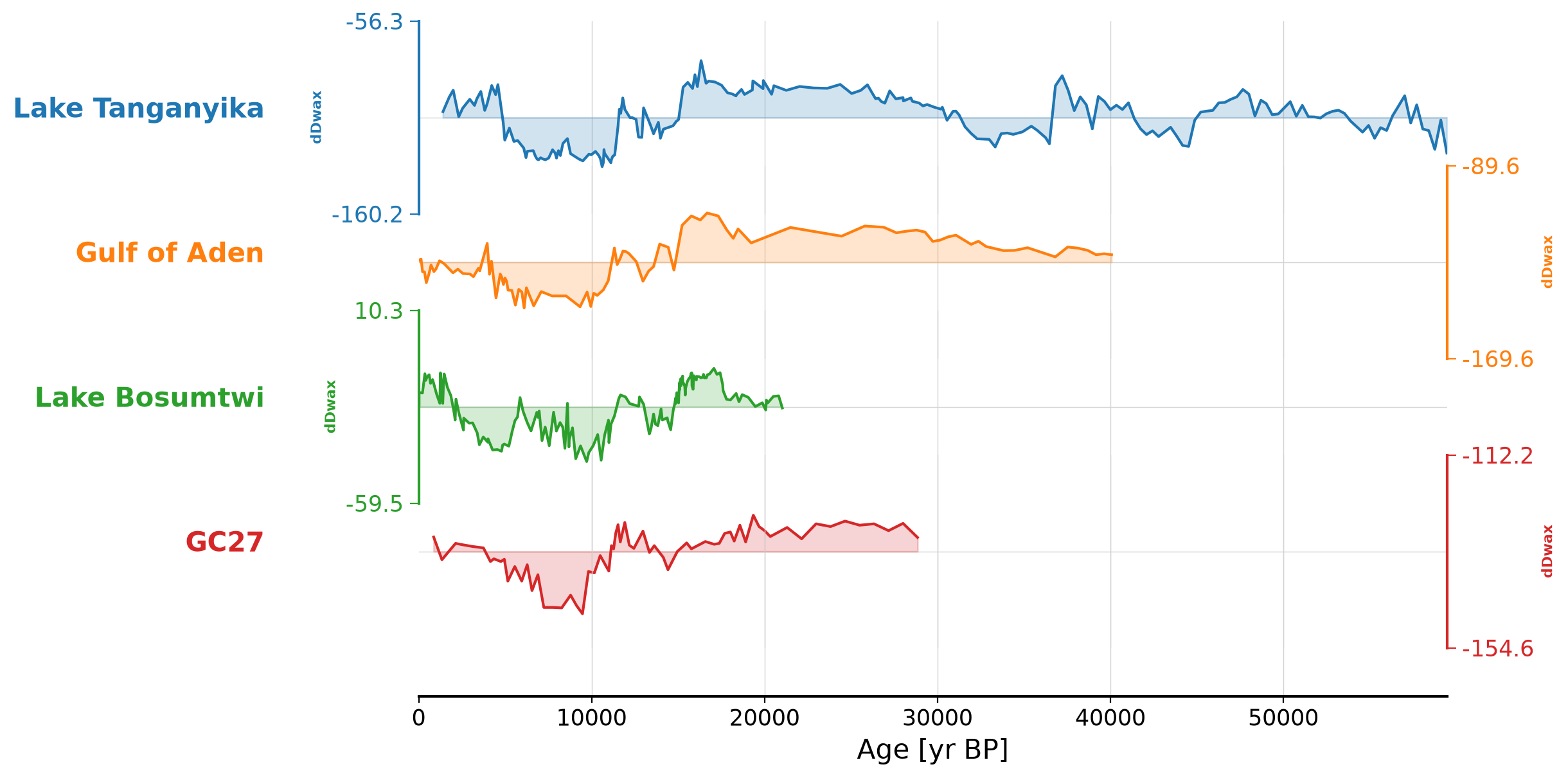
By creating a stackplot, we can visually compare between the datasets. However, the four δD records aren’t the same resolution and don’t span the same time interval.
To better compare the records and assess a common trend, we can use PCA. First, we can use .common_time() to place the records on a shared time axis with a common sampling frequency. This function takes the argument method, which can be either bin, interp, and gdkernel. The binning and interpolation methods are what we just covered in the previous section. Let’s set the time step to 500 years, the method to interp, and standardize the data:
africa_ct = ms_africa.common_time(method="interp", step=0.5).standardize()
fig, ax = africa_ct.stackplot()
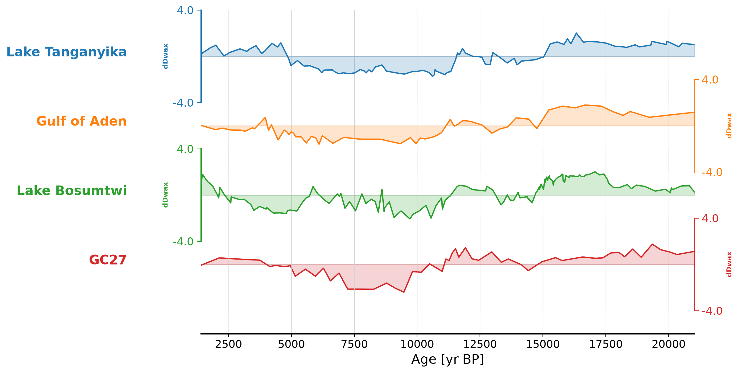
We now have standardized δD records that are the same sampling resolution and span the same time interval. Note this meant trimming the longer time series down to around 20,000 years in length.
We can now apply PCA which will allow us to quantitatively identify a common signal between the four δD paleoclimate reconstructions through the .pca() method.
The pyleoclim package has its own pca method ( e.g. africa_ct.pca()), but it is computationally intensive for use in this course. For our purposes we will be using the PCA method from sklearn. Please refer to this example for further reference.
pca = PCA()
africa_PCA = pca.fit(africa_ct.to_pandas())
The result is an object containing multiple outputs. The two outputs we’ll look at is the percentage of variance accounted for by each mode as well as the principal components themselves.
First, let’s print the percentage of variance accounted for by each mode, noting that the first principle component is first in the list, and so on.
print(africa_PCA.explained_variance_ratio_)
[0.79710569 0.11020624 0.05970267 0.0329854 ]
This means that most of the variance in the four paleoclimate records is explained by the first principal component (the first value displayed). The number of datasets in the PCA constrains the number of principal components that can be defined, which is why we only have four components in this example.
We can now look at the principal component of the first mode of variance. Let’s create a new series for the first principle component and plot it against the original datasets:
africa_pc1 = africa_PCA.transform(africa_ct.to_pandas())
africa_mode1 = pyleo.Series(
    time=africa_ct.series_list[0].time,
    value=africa_pc1[:,0],
    label=r'$PC_1$',
    value_name='PC1',
    time_name ='age',
    time_unit = 'yr BP'
)
Time axis values sorted in ascending order
fig, ax1 = plt.subplots()

ax1.set_ylabel("dDwax")
ax2 = ax1.twinx()  # instantiate a second axes that shares the same x-axis
ax2.set_ylabel("PC1")  # we already handled the x-label with ax1

# plt.plot(mode1.time,pc1_scaled)
africa_mode1.plot(color="black", ax=ax2, invert_yaxis=True)
africa_ct.plot(ax=ax1, linewidth=0.5)
<Axes: title={'center': 'African dDwax'}, xlabel='Age [yr BP]', ylabel='dDwax'>
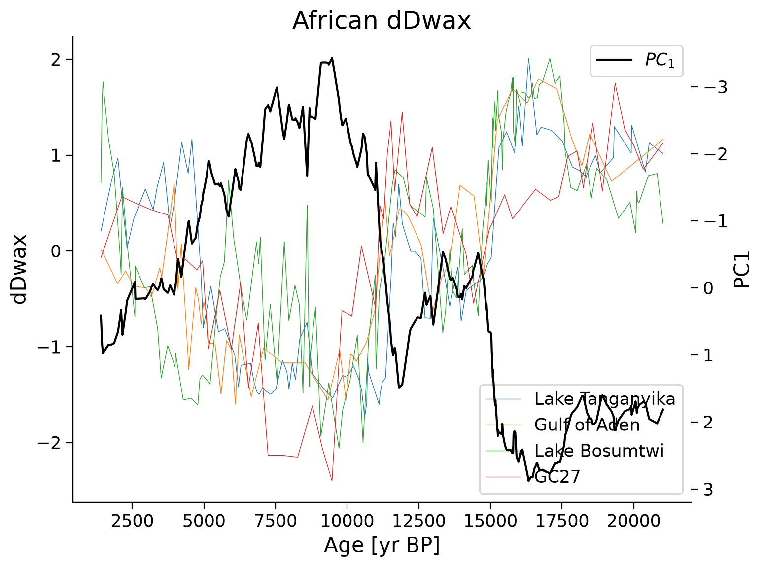
The original δD records are shown in the colored lines, and the first principal component (PC1) time series is shown in black.
Questions 3: Climate Connection#
How do the original time series compare to the PC1 time series? Do they record similar trends?
Which original δD record most closely resembles the PC1 time series? Which is the most different?
What changes in climate does the PC1 time series record over the past 20,000 years? Hint: remember that more depleted (more negative) δD suggests increased rainfall.
Submit your feedback#
Show code cell source
# @title Submit your feedback
content_review(f"{feedback_prefix}_Questions_3")
Summary#
In this tutorial, you explored a variety of computational techniques for analyzing paleoclimate data. You learned how to handle irregular data and place these records on a uniform time axis using interpolation and binning.
You then explored Principal Component Analysis (PCA), a method that reveals common signals across various paleoclimate reconstructions. To effectively utilize PCA, it’s essential to have all records on the same sampling resolution and same time step, which can be achieved using the resampling tools you learned in this tutorial.
For your practical example, we used a dataset of hydrogen isotopes of leaf waxes (δDwax) from Lake Tanganyika in East Africa to further enhance your understanding of the discussed techniques, equipping you to better analyze and understand the complexities of paleoclimate data.
Resources#
Code for this tutorial is based on existing notebooks from LinkedEarth for anlayzing LiPD datasets and resampling data with Pyleoclim.
Data from the following sources are used in this tutorial:
Tierney, J.E., et al. 2008. Northern Hemisphere Controls on Tropical Southeast African Climate During the Past 60,000 Years. Science, Vol. 322, No. 5899, pp. 252-255, 10 October 2008. https://doi.org/10.1126/science.1160485.
Tierney, J.E., and deMenocal, P.. 2013. Abrupt Shifts in Horn of Africa Hydroclimate Since the Last Glacial Maximum. Science, 342(6160), 843-846. https://doi.org/10.1126/science.1240411.
Tierney, J.E., Pausata, F., deMenocal, P. 2017. Rainfall Regimes of the Green Sahara. Science Advances, 3(1), e1601503. https://doi.org/10.1126/sciadv.1601503.
Shanahan, T.M., et al. 2015. The time-transgressive termination of the African Humid Period. Nature Geoscience, 8(2), 140-144. https://doi.org/10.1038/ngeo2329.