Tutorial 3: Reconstructing Past Changes in Terrestrial Climate

Tutorial 3: Reconstructing Past Changes in Terrestrial Climate#

Week 1, Day 4, Paleoclimate

Content creators: Sloane Garelick

Content reviewers: Yosmely Bermúdez, Dionessa Biton, Katrina Dobson, Maria Gonzalez, Will Gregory, Nahid Hasan, Paul Heubel, Sherry Mi, Beatriz Cosenza Muralles, Brodie Pearson, Jenna Pearson, Chi Zhang, Ohad Zivan

Content editors: Yosmely Bermúdez, Paul Heubel, Zahra Khodakaramimaghsoud, Jenna Pearson, Agustina Pesce, Chi Zhang, Ohad Zivan

Production editors: Wesley Banfield, Paul Heubel, Jenna Pearson, Konstantine Tsafatinos, Chi Zhang, Ohad Zivan

Our 2024 Sponsors: CMIP, NFDI4Earth

Tutorial Objectives#

Estimated timing of tutorial: 20 minutes

In this tutorial, we’ll explore the Euro2K proxy network, which is a subset of PAGES2K, the database we explored in the first tutorial. We will specifically focus on interpreting temperature change over the past 2,000 years as recorded by proxy records from tree rings, speleothems, and lake sediments. To analyze these datasets, we will group them by archive and create time series plots to assess temperature variations.

During this tutorial, you will:

Plot temperature records based on three different terrestrial proxies
Assess similarities and differences between the temperature records

Setup#

# installations ( uncomment and run this cell ONLY when using google colab or kaggle )

# !pip install LiPD
# !pip install cartopy
# !pip install pyleoclim

# imports
import pyleoclim as pyleo
import pandas as pd
import numpy as np
import os
import pooch
import tempfile
import matplotlib.pyplot as plt
import cartopy.crs as ccrs
import cartopy.feature as cfeature
from io import StringIO
import sys

Figure Settings#

Helper functions#

Video 1: Terrestrial Climate Proxies#

Section 1: Loading Terrestrial Paleoclimate Records#

First, we need to download the data. Similar to Tutorial 1, the data is stored as a LiPD file, and we will be using Pyleoclim to format and interpret the data.

# set the name to save the Euro2k data
fname = "euro2k_data"

# download the data
lipd_file_path = pooch.retrieve(
    url="https://osf.io/7ezp3/download/",
    known_hash=None,
    path="./",
    fname=fname,
    processor=pooch.Unzip(),
)

Downloading data from 'https://osf.io/7ezp3/download/' to file '/home/runner/work/climate-course-content/climate-course-content/tutorials/W1D4_Paleoclimate/student/euro2k_data'.

SHA256 hash of downloaded file: 55246ce189fd3620cb1467f3c558c22ce91be368fabde3f0c2aeb18551c9d5be
Use this value as the 'known_hash' argument of 'pooch.retrieve' to ensure that the file hasn't changed if it is downloaded again in the future.

Unzipping contents of '/home/runner/work/climate-course-content/climate-course-content/tutorials/W1D4_Paleoclimate/student/euro2k_data' to '/home/runner/work/climate-course-content/climate-course-content/tutorials/W1D4_Paleoclimate/student/euro2k_data.unzip'

# the LiPD object can be used to load datasets stored in the LiPD format.
# in this first case study, we will load an entire library of LiPD files:
with SupressOutputs():
    d_euro = pyleo.Lipd(os.path.join(".", f"{fname}.unzip", "Euro2k"))

---------------------------------------------------------------------------
AttributeError                            Traceback (most recent call last)
Cell In[8], line 4
      1 # the LiPD object can be used to load datasets stored in the LiPD format.
      2 # in this first case study, we will load an entire library of LiPD files:
      3 with SupressOutputs():
----> 4     d_euro = pyleo.Lipd(os.path.join(".", f"{fname}.unzip", "Euro2k"))

AttributeError: module 'pyleoclim' has no attribute 'Lipd'

Section 2: Temperature Reconstructions#

Before plotting, let’s narrow the data down a bit. We can filter all of the data so that we only keep reconstructions of temperature from terrestrial archives (e.g. tree rings, speleothems and lake sediments). This is accomplished with the function below.

def filter_data(dataset, archive_type, variable_name):
    """
    Return a MultipleSeries object with the variable record (variable_name) for a given archive_type and coordinates.
    """
    # Create a list of dictionary that can be iterated upon using Lipd.to_tso method
    ts_list = dataset.to_tso()
    # Append the correct indices for a given value of archive_type and variable_name
    indices = []
    lat = []
    lon = []
    for idx, item in enumerate(ts_list):
        # Check that it is available to avoid errors on the loop
        if "archiveType" in item.keys():
            # If it's a archive_type, then proceed to the next step
            if item["archiveType"] == archive_type:
                if item["paleoData_variableName"] == variable_name:
                    indices.append(idx)
    print(indices)
    # Create a list of LipdSeries for the given indices
    ts_list_archive_type = []
    for indice in indices:
        ts_list_archive_type.append(pyleo.LipdSeries(ts_list[indice]))

        # save lat and lons of proxies
        lat.append(ts_list[indice]["geo_meanLat"])
        lon.append(ts_list[indice]["geo_meanLon"])

    return pyleo.MultipleSeries(ts_list_archive_type), lat, lon

In the function above, the Lipd.to_tso() method is used to obtain a list of dictionaries that can be iterated upon.

ts_list = d_euro.to_tso()

Dictionaries are native to Python and can be explored as shown below.

# look at available entries for just one time-series
ts_list[0].keys()

# print relevant information for all entries
for idx, item in enumerate(ts_list):
    print(str(idx) + ": " + item["dataSetName"] +
          ": " + item["paleoData_variableName"])

Now let’s use our pre-defined function to create a new list that only has temperature reconstructions based on proxies from lake sediments:

ms_euro_lake, euro_lake_lat, euro_lake_lon = filter_data(
    d_euro, "lake sediment", "temperature"
)

And a new list that only has temperature reconstructions based on proxies from tree rings:

ms_euro_tree, euro_tree_lat, euro_tree_lon = filter_data(
    d_euro, "tree", "temperature")

And finally, a new list that only has temperature information based on proxies from speleothems:

ms_euro_spel, euro_spel_lat, euro_spel_lon = filter_data(
    d_euro, "speleothem", "d18O")

Coding Exercises 2#

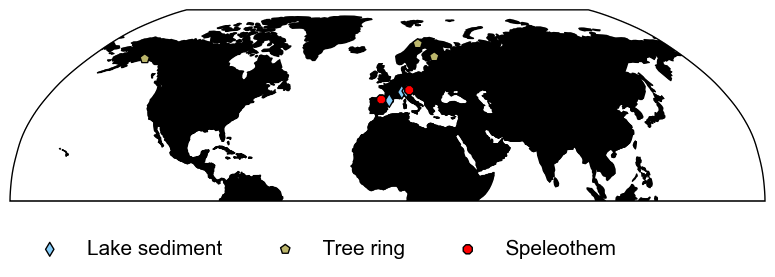
Using the coordinate information output from the filter_data() function, make a plot of the locations of the proxies using the markers and colors from Tutorial 1. Note that data close together may not be very visible.

# initiate plot
fig = plt.figure()

# set base map projection
ax = plt.axes(projection=ccrs.Robinson())

ax.set_global()

# add land fratures using gray color
ax.add_feature(cfeature.LAND, facecolor="k")

# add coastlines
ax.add_feature(cfeature.COASTLINE)

#################################################
## TODO for students: add the proxy locations ##
# Remove or comment the following line of code once you have completed the exercise:
raise NotImplementedError("Student exercise: Add the proxy locations via a scatter plot method.")
#################################################
# add the proxy locations
_ = ax.scatter(
    ...,
    ...,
    transform=ccrs.Geodetic(),
    label=...,
    s=50,
    marker="d",
    color=[0.52734375, 0.8046875, 0.97916667],
    edgecolor="k",
    zorder=2,
)
_ = ax.scatter(
    ...,
    ...,
    transform=ccrs.Geodetic(),
    label=...,
    s=50,
    marker="p",
    color=[0.73828125, 0.71484375, 0.41796875],
    edgecolor="k",
    zorder=2,
)
_ = ax.scatter(
    ...,
    ...,
    transform=ccrs.Geodetic(),
    label=...,
    s=50,
    marker="8",
    color=[1, 0, 0],
    edgecolor="k",
    zorder=2,
)

# change the map view to zoom in on central Pacific
ax.set_extent((0, 360, 0, 90), crs=ccrs.PlateCarree())

ax.legend(
    scatterpoints=1,
    bbox_to_anchor=(0, -0.4),
    loc="lower left",
    ncol=3,
    fontsize=15,
)

Click for solution

Example output:

Since we are going to compare temperature datasets based on different terrestrial climate archives (lake sediments, tree rings and speleothems), the quantitative values of the measurements in each record will differ (i.e., the lake sediment and tree ring data are temperature in degrees C, but the speleothem data is oxygen isotopes in per mille). Therefore, to more easily and accurately compare temperature between the records, it’s helpful to standardize the data as we did in Tutorial 2. The .standardize() function removes the estimated mean of the time series and divides by its estimated standard deviation.

# standardize the data
spel_stnd = ms_euro_spel.standardize()
lake_stnd = ms_euro_lake.standardize()
tree_stnd = ms_euro_tree.standardize()

Now we can use Pyleoclim functions to create three stacked plots of this data with lake sediment records on top, tree ring reconstructions in the middle and speleothem records on the bottom.

Note that the colors used for the time series in each plot are the default colors generated by the function, so the corresponding colors in each of the three plots are not relevant.

# note the x-axis is years before present,
# so reading from left to right corresponds to moving back in time

ax = lake_stnd.stackplot(
    label_x_loc=1.7,
    xlim=[0, 2000],
    v_shift_factor=1,
    figsize=[9, 5],
    time_unit="yrs BP",
)
ax[0].suptitle("Lake Cores", y=1.2)

ax = tree_stnd.stackplot(
    label_x_loc=1.7,
    xlim=[0, 2000],
    v_shift_factor=1,
    figsize=[9, 5],
    time_unit="yrs BP",
)
ax[0].suptitle("Tree Rings", y=1.2)

# recall d18O is a proxy for SST, and that more positive d18O means colder SST
ax = spel_stnd.stackplot(
    label_x_loc=1.7,
    xlim=[0, 2000],
    v_shift_factor=1,
    figsize=[9, 5],
    time_unit="yrs BP",
)
ax[0].suptitle("Speleothems", y=1.2)

Questions 2#

Using the plots we just made (and recalling that all of these records are from Europe), let’s make some inferences about the temperature data over the past 2,000 years:

Recall that δ¹⁸O is a proxy for SST, and that more positive δ¹⁸O means colder SST. Do the temperature records based on a single proxy type record similar patterns?
Do the three proxy types collectively record similar patterns?
What might be causing the more frequent variations in temperature?