![]()

Tutorial 5: Testing generalization to new scenarios#
Week 2, Day 5, AI and Climate Change
Content creators: Deepak Mewada, Grace Lindsay
Content reviewers: Mujeeb Abdulfatai, Nkongho Ayuketang Arreyndip, Jeffrey N. A. Aryee, Paul Heubel, Jenna Pearson, Abel Shibu
Content editors: Deepak Mewada, Grace Lindsay
Production editors: Konstantine Tsafatinos
Our 2024 Sponsors: CMIP, NFDI4Earth
Tutorial Objectives#
Estimated timing of tutorial: 20 minutes
In this tutorial, you will
Learn about a different type of out-of-distribution test of our model
Evaluate the model’s performance
Setup#
# imports

import matplotlib.pyplot as plt                           # For plotting graphs
import pandas as pd                                       # For data manipulation
# # Import specific machine learning models and tools
from sklearn.model_selection import train_test_split      # For splitting dataset into train and test sets
from sklearn.ensemble import RandomForestRegressor        # For Random Forest Regression
Figure Settings#
Show code cell source
# @title Figure Settings
import ipywidgets as widgets  # interactive display

%config InlineBackend.figure_format = 'retina'
plt.style.use(
    "https://raw.githubusercontent.com/neuromatch/climate-course-content/main/cma.mplstyle"
)
Helper functions#
Show code cell source
# @title Helper functions

# Load and Prepare the Data
url_Climatebench_train_val = "https://osf.io/y2pq7/download"  # Dataset URL
training_data = pd.read_csv(url_Climatebench_train_val)  # load the training data from the provided URL
training_data.pop('scenario')  # drop the 'scenario' column as it's just a label and won't be passed into the model
target = training_data.pop('tas_FINAL')  # extract the target variable 'tas_FINAL' which we aim to predict

url_spatial_test_data = "https://osf.io/7tr49/download" # test data with different location
spatial_test_data = pd.read_csv(url_spatial_test_data)  # load spatial test data from the provided URL
spatial_test_data.pop('scenario')  # drop the `scenario` column from the data as it is just a label, but will not be passed into the model.
spatial_test_target = spatial_test_data.pop('tas_FINAL')  # extract the target variable 'tas_FINAL'

# Split the data into training and testing sets: 80%/20%
X_train, X_test, y_train, y_test = train_test_split(training_data, target, test_size=0.2, random_state=1)

# Training the model on the training data
rf_regressor = RandomForestRegressor(random_state=42, n_estimators=80, max_depth=50)
rf_regressor.fit(X_train, y_train)

spatial_test_score = rf_regressor.score(spatial_test_data,spatial_test_target)
Set random seed#
Executing set_seed(seed=seed) you are setting the seed
Show code cell source
# @title Set random seed

# @markdown Executing `set_seed(seed=seed)` you are setting the seed

# Call `set_seed` function in the exercises to ensure reproducibility.
import random
import numpy as np

def set_seed(seed=None):
    if seed is None:
        seed = np.random.choice(2 ** 32)
    random.seed(seed)
    np.random.seed(seed)
    print(f'Random seed {seed} has been set.')

# Set a global seed value for reproducibility
random_state = 42 # change 42 with any number you like

set_seed(seed=random_state)
Random seed 42 has been set.
Video 1: Testing generalization to new scenarios#
Video Summary :
Discussed how we previously tested generalization to an unseen region.
Stressed that the real utility of these emulators is the ability to run new scenarios.
Now we will see if the model generalizes to data from a new scenario.
Section 1: Test Generalization to Held-out Emissions Scenario#
Section 1.1: Load the New Testing (Scenario) Data#
Load the new dataset and print it. As you can see, the scenario for all of these datapoints is ssp245. This scenario was not included in our initial data set. According to the scenario descriptions included in the table in Tutorial 1, ssp245 represent a “medium forcing future scenario”. The lat/lon locations are the same as the initial dataset (blue box region).
url_scenario_test_data = "https://osf.io/pkbwx/download"  # Dataset URL
scenario_test_data = pd.read_csv(url_scenario_test_data)  # Load scenario test data from the provided URL
scenario_test_data
| scenario | lat | lon | tas_2015 | pr_2015 | pr90_2015 | dtr_2015 | tas_FINAL | CO2_2015 | SO2_2015 | ... | CH4_2048 | BC_2048 | CO2_2049 | SO2_2049 | CH4_2049 | BC_2049 | CO2_2050 | SO2_2050 | CH4_2050 | BC_2050 | |
|---|---|---|---|---|---|---|---|---|---|---|---|---|---|---|---|---|---|---|---|---|---|
| 0 | ssp245 | -19.894737 | 0.0 | 0.555990 | -9.931833e-08 | -3.426345e-07 | -0.042485 | 0.839935 | 1536.072222 | 6.686393e-08 | ... | 0.347418 | 3.033223e-09 | 2907.777226 | 3.432615e-08 | 0.344846 | 2.978194e-09 | 2950.734869 | 3.345217e-08 | 0.342274 | 2.923164e-09 |
| 1 | ssp245 | -19.894737 | 2.5 | 0.547587 | -2.084760e-07 | -5.129149e-07 | -0.055545 | 0.800608 | 1536.072222 | 6.686393e-08 | ... | 0.347418 | 3.033223e-09 | 2907.777226 | 3.432615e-08 | 0.344846 | 2.978194e-09 | 2950.734869 | 3.345217e-08 | 0.342274 | 2.923164e-09 |
| 2 | ssp245 | -19.894737 | 5.0 | 0.476858 | -3.123266e-07 | -7.148436e-07 | -0.065286 | 0.739756 | 1536.072222 | 6.686393e-08 | ... | 0.347418 | 3.033223e-09 | 2907.777226 | 3.432615e-08 | 0.344846 | 2.978194e-09 | 2950.734869 | 3.345217e-08 | 0.342274 | 2.923164e-09 |
| 3 | ssp245 | -19.894737 | 7.5 | 0.309591 | -1.828261e-07 | -8.008969e-07 | -0.044665 | 0.824819 | 1536.072222 | 6.686393e-08 | ... | 0.347418 | 3.033223e-09 | 2907.777226 | 3.432615e-08 | 0.344846 | 2.978194e-09 | 2950.734869 | 3.345217e-08 | 0.342274 | 2.923164e-09 |
| 4 | ssp245 | -19.894737 | 10.0 | 0.169423 | -6.493187e-08 | -7.357342e-07 | -0.024194 | 0.984558 | 1536.072222 | 6.686393e-08 | ... | 0.347418 | 3.033223e-09 | 2907.777226 | 3.432615e-08 | 0.344846 | 2.978194e-09 | 2950.734869 | 3.345217e-08 | 0.342274 | 2.923164e-09 |
| ... | ... | ... | ... | ... | ... | ... | ... | ... | ... | ... | ... | ... | ... | ... | ... | ... | ... | ... | ... | ... | ... |
| 805 | ssp245 | 63.473684 | 32.5 | 0.084310 | 1.681694e-06 | 4.141917e-06 | -0.530416 | 1.196798 | 1536.072222 | 6.686393e-08 | ... | 0.347418 | 3.033223e-09 | 2907.777226 | 3.432615e-08 | 0.344846 | 2.978194e-09 | 2950.734869 | 3.345217e-08 | 0.342274 | 2.923164e-09 |
| 806 | ssp245 | 63.473684 | 35.0 | 0.081848 | 1.380857e-06 | 3.192422e-06 | -0.447510 | 1.191854 | 1536.072222 | 6.686393e-08 | ... | 0.347418 | 3.033223e-09 | 2907.777226 | 3.432615e-08 | 0.344846 | 2.978194e-09 | 2950.734869 | 3.345217e-08 | 0.342274 | 2.923164e-09 |
| 807 | ssp245 | 63.473684 | 37.5 | 0.215474 | 1.626266e-06 | 5.394675e-06 | -0.503612 | 1.192739 | 1536.072222 | 6.686393e-08 | ... | 0.347418 | 3.033223e-09 | 2907.777226 | 3.432615e-08 | 0.344846 | 2.978194e-09 | 2950.734869 | 3.345217e-08 | 0.342274 | 2.923164e-09 |
| 808 | ssp245 | 63.473684 | 40.0 | 0.174184 | 1.313737e-06 | 5.731348e-06 | -0.659323 | 1.157979 | 1536.072222 | 6.686393e-08 | ... | 0.347418 | 3.033223e-09 | 2907.777226 | 3.432615e-08 | 0.344846 | 2.978194e-09 | 2950.734869 | 3.345217e-08 | 0.342274 | 2.923164e-09 |
| 809 | ssp245 | 63.473684 | 42.5 | 0.174011 | 8.657128e-07 | 2.236403e-06 | -0.479017 | 1.250509 | 1536.072222 | 6.686393e-08 | ... | 0.347418 | 3.033223e-09 | 2907.777226 | 3.432615e-08 | 0.344846 | 2.978194e-09 | 2950.734869 | 3.345217e-08 | 0.342274 | 2.923164e-09 |
810 rows × 152 columns
Now we will prepare the data to be fed into the pre-trained model.
scenario_test_data.pop('scenario')  # remove the 'scenario' column from the dataset
scenario_test_target = scenario_test_data.pop('tas_FINAL')  # extract the target variable 'tas_FINAL'
scenario_test_data  # display the prepared scenario test data
| lat | lon | tas_2015 | pr_2015 | pr90_2015 | dtr_2015 | CO2_2015 | SO2_2015 | CH4_2015 | BC_2015 | ... | CH4_2048 | BC_2048 | CO2_2049 | SO2_2049 | CH4_2049 | BC_2049 | CO2_2050 | SO2_2050 | CH4_2050 | BC_2050 | |
|---|---|---|---|---|---|---|---|---|---|---|---|---|---|---|---|---|---|---|---|---|---|
| 0 | -19.894737 | 0.0 | 0.555990 | -9.931833e-08 | -3.426345e-07 | -0.042485 | 1536.072222 | 6.686393e-08 | 0.373737 | 5.090832e-09 | ... | 0.347418 | 3.033223e-09 | 2907.777226 | 3.432615e-08 | 0.344846 | 2.978194e-09 | 2950.734869 | 3.345217e-08 | 0.342274 | 2.923164e-09 |
| 1 | -19.894737 | 2.5 | 0.547587 | -2.084760e-07 | -5.129149e-07 | -0.055545 | 1536.072222 | 6.686393e-08 | 0.373737 | 5.090832e-09 | ... | 0.347418 | 3.033223e-09 | 2907.777226 | 3.432615e-08 | 0.344846 | 2.978194e-09 | 2950.734869 | 3.345217e-08 | 0.342274 | 2.923164e-09 |
| 2 | -19.894737 | 5.0 | 0.476858 | -3.123266e-07 | -7.148436e-07 | -0.065286 | 1536.072222 | 6.686393e-08 | 0.373737 | 5.090832e-09 | ... | 0.347418 | 3.033223e-09 | 2907.777226 | 3.432615e-08 | 0.344846 | 2.978194e-09 | 2950.734869 | 3.345217e-08 | 0.342274 | 2.923164e-09 |
| 3 | -19.894737 | 7.5 | 0.309591 | -1.828261e-07 | -8.008969e-07 | -0.044665 | 1536.072222 | 6.686393e-08 | 0.373737 | 5.090832e-09 | ... | 0.347418 | 3.033223e-09 | 2907.777226 | 3.432615e-08 | 0.344846 | 2.978194e-09 | 2950.734869 | 3.345217e-08 | 0.342274 | 2.923164e-09 |
| 4 | -19.894737 | 10.0 | 0.169423 | -6.493187e-08 | -7.357342e-07 | -0.024194 | 1536.072222 | 6.686393e-08 | 0.373737 | 5.090832e-09 | ... | 0.347418 | 3.033223e-09 | 2907.777226 | 3.432615e-08 | 0.344846 | 2.978194e-09 | 2950.734869 | 3.345217e-08 | 0.342274 | 2.923164e-09 |
| ... | ... | ... | ... | ... | ... | ... | ... | ... | ... | ... | ... | ... | ... | ... | ... | ... | ... | ... | ... | ... | ... |
| 805 | 63.473684 | 32.5 | 0.084310 | 1.681694e-06 | 4.141917e-06 | -0.530416 | 1536.072222 | 6.686393e-08 | 0.373737 | 5.090832e-09 | ... | 0.347418 | 3.033223e-09 | 2907.777226 | 3.432615e-08 | 0.344846 | 2.978194e-09 | 2950.734869 | 3.345217e-08 | 0.342274 | 2.923164e-09 |
| 806 | 63.473684 | 35.0 | 0.081848 | 1.380857e-06 | 3.192422e-06 | -0.447510 | 1536.072222 | 6.686393e-08 | 0.373737 | 5.090832e-09 | ... | 0.347418 | 3.033223e-09 | 2907.777226 | 3.432615e-08 | 0.344846 | 2.978194e-09 | 2950.734869 | 3.345217e-08 | 0.342274 | 2.923164e-09 |
| 807 | 63.473684 | 37.5 | 0.215474 | 1.626266e-06 | 5.394675e-06 | -0.503612 | 1536.072222 | 6.686393e-08 | 0.373737 | 5.090832e-09 | ... | 0.347418 | 3.033223e-09 | 2907.777226 | 3.432615e-08 | 0.344846 | 2.978194e-09 | 2950.734869 | 3.345217e-08 | 0.342274 | 2.923164e-09 |
| 808 | 63.473684 | 40.0 | 0.174184 | 1.313737e-06 | 5.731348e-06 | -0.659323 | 1536.072222 | 6.686393e-08 | 0.373737 | 5.090832e-09 | ... | 0.347418 | 3.033223e-09 | 2907.777226 | 3.432615e-08 | 0.344846 | 2.978194e-09 | 2950.734869 | 3.345217e-08 | 0.342274 | 2.923164e-09 |
| 809 | 63.473684 | 42.5 | 0.174011 | 8.657128e-07 | 2.236403e-06 | -0.479017 | 1536.072222 | 6.686393e-08 | 0.373737 | 5.090832e-09 | ... | 0.347418 | 3.033223e-09 | 2907.777226 | 3.432615e-08 | 0.344846 | 2.978194e-09 | 2950.734869 | 3.345217e-08 | 0.342274 | 2.923164e-09 |
810 rows × 150 columns
Section 1.2: Evaluate the Model on this New (Scenario) Data#
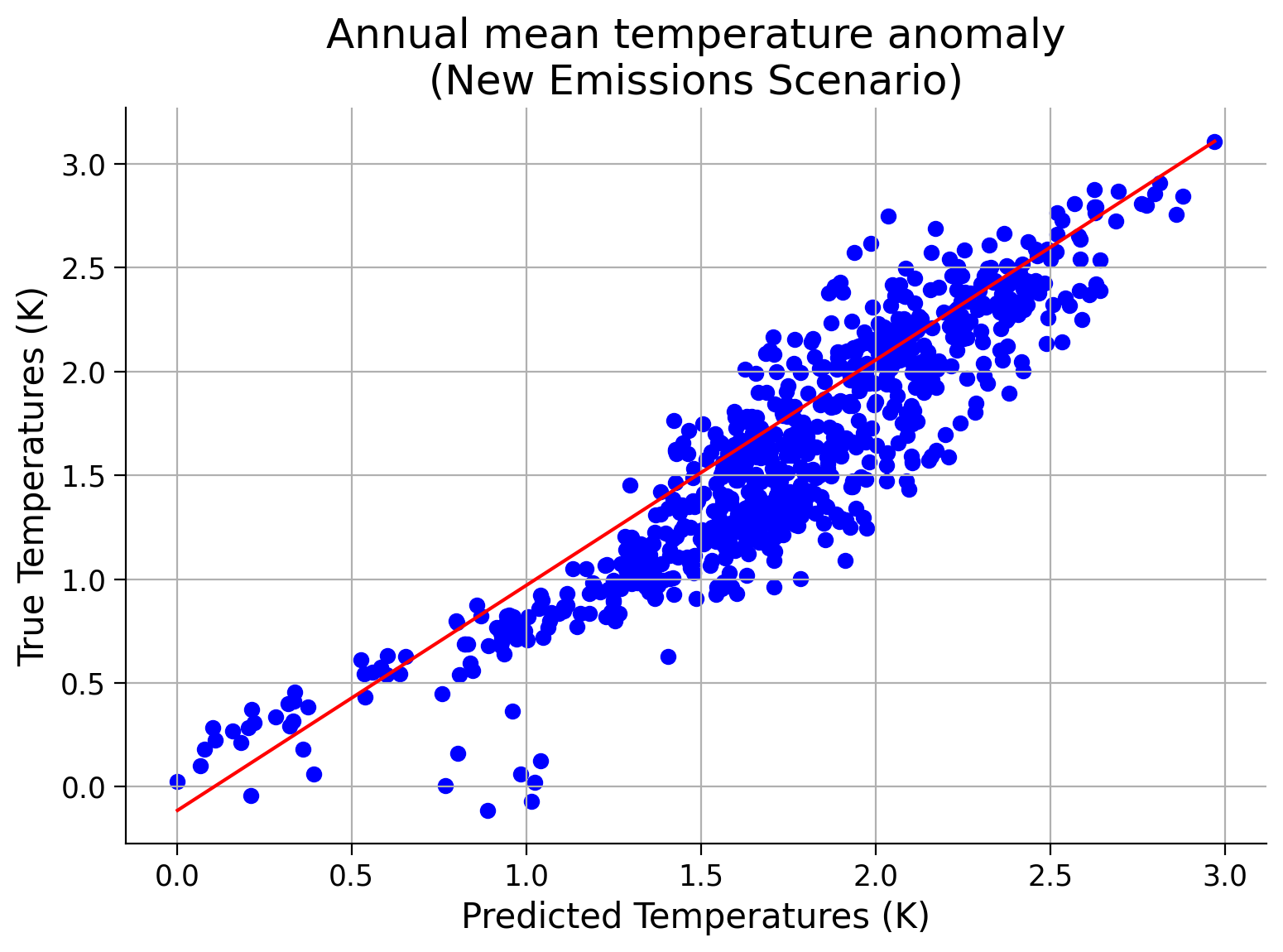
Now let’s evaluate our pre-trained model (rf_regressor) to see how well it performs on this new emissions scenario. Use what you know to evaluate the performance and make a scatter plot of predicted vs. true temperature values.
def evaluate_and_plot_scenario_performance(rf_regressor, scenario_test_data, scenario_test_target):
    """Evaluate the performance of the pre-trained model on the new emissions scenario
    and create a scatter plot of predicted vs. true temperature values.

    Args:
        rf_regressor (RandomForestRegressor): Pre-trained Random Forest regressor model.
        scenario_test_data (ndarray): Test features for the new emissions scenario.
        scenario_test_target (ndarray): True temperature values of the new emissions scenario.

    Returns:
        float: Score of the model on the scenario test data.
    """

    # predict temperature values for the new emissions scenario
    scenario_test_predicted = ...

    # evaluate the model on the new emissions scenario
    scenario_test_score = ...
    print("Scenario Test Score:", scenario_test_score)

    # implement plt.scatter() to compare predicted and true temperature values
    plt.figure()
    _ = ...
    # implement plt.plot() to plot the diagonal line y=x
    _ = ...

    # aesthetics
    plt.xlabel('Predicted Temperatures (K)')
    plt.ylabel('True Temperatures (K)')
    plt.title('Annual mean temperature anomaly\n(New Emissions Scenario)')
    plt.grid(True)
    plt.show()

    return scenario_test_score

# test your function
scenario_test_score = evaluate_and_plot_scenario_performance(rf_regressor, scenario_test_data, scenario_test_target)
Scenario Test Score: Ellipsis
Example output:
Question 1.2: Performance of the Model on New Scenario Data#
Again, have you observed a decrease in the score?
What do you believe could be the cause of this?
What kind of new scenarios might the model perform better for?
For the sake of clarity let’s summarize all the result.
# summarize results
train_score = rf_regressor.score(X_train, y_train)
test_score  = rf_regressor.score(X_test, y_test)
average_score = (train_score + test_score + spatial_test_score + scenario_test_score) / 4

print(f"\tTraining Data Score                             : {train_score}")
print(f"\tTesting Data Score on same Scenario/Region      : {test_score}")
print(f"\tHeld-out Spatial Region Test Score              : {spatial_test_score}")
print(f"\tHeld-out Scenario Test Score                    : {scenario_test_score}")
---------------------------------------------------------------------------
TypeError                                 Traceback (most recent call last)
Cell In[10], line 4
      2 train_score = rf_regressor.score(X_train, y_train)
      3 test_score  = rf_regressor.score(X_test, y_test)
----> 4 average_score = (train_score + test_score + spatial_test_score + scenario_test_score) / 4
      6 print(f"\tTraining Data Score                             : {train_score}")
      7 print(f"\tTesting Data Score on same Scenario/Region      : {test_score}")

TypeError: unsupported operand type(s) for +: 'float' and 'ellipsis'
This shows us that the model does generalize somewhat (i.e. the score is well above zero even in the new regions and in the new scenario). However, it does not generalize very well. That is, it does not perform as well on data that differs from the data it was trained on. Ideally, we would be able to build a model that inherently learns the complex relationship between emissions scenarios and future temperature. A model that truly learned this relationship would be able to generalize to new scenarios and regions.
Do you have any ideas of how to build a better machine learning model to emulate climate models? Many scientists are working on this problem!
Bonus Section 2: Try other Regression Models#
Only complete this section if you are well ahead of schedule, or have already completed the final tutorial.
Random Forest models are not the only regression models that could be applied to this problem. In this code, we will use scikit-learn to train and evaluate various regression models on the Climate Bench dataset. We will load the data, split it, define models, train them with different settings, and evaluate their performance. We will calculate and print average scores for each model configuration and identify the best-performing model.
For more information about the models used here and various other models, you can refer to scikit-learn.org/stable/supervised_learning.html#supervised-learning.
Note: the following cell may take ~2 minutes to run.
# Import necessary libraries
import matplotlib.pyplot as plt
from sklearn.pipeline import make_pipeline
from sklearn.preprocessing import StandardScaler
from sklearn.model_selection import train_test_split
from sklearn.ensemble import RandomForestRegressor, GradientBoostingRegressor, BaggingRegressor
from sklearn.svm import SVR
from sklearn.linear_model import LinearRegression, Ridge, Lasso, ElasticNet
from sklearn.linear_model import RidgeCV
import pandas as pd
from sklearn.neural_network import MLPRegressor

# Load datasets
train_val_data = pd.read_csv("https://osf.io/y2pq7/download")
spatial_test_data = pd.read_csv("https://osf.io/7tr49/download")
scenario_test_data = pd.read_csv("https://osf.io/pkbwx/download")

# Pop the 'scenario' column from all datasets
train_val_data.pop('scenario')
spatial_test_data.pop('scenario')
scenario_test_data.pop('scenario')

# Split train_val_data into training and testing sets
X_train, X_test, y_train, y_test = train_test_split(train_val_data.drop(columns=["tas_FINAL"]),
                                                    train_val_data["tas_FINAL"],
                                                    test_size=0.2,
                                                    random_state=1)

# Define models with different configurations
models = {
    "MLP": [make_pipeline(StandardScaler(), MLPRegressor(hidden_layer_sizes=(50,), max_iter=1000)),
            make_pipeline(StandardScaler(), MLPRegressor(hidden_layer_sizes=(500, 500, 500), random_state=1, max_iter=1000))],
    "RandomForest": [make_pipeline(StandardScaler(), RandomForestRegressor(n_estimators=100, max_depth=None)),
                     make_pipeline(StandardScaler(), RandomForestRegressor(n_estimators=50, max_depth=10))],
    "GradientBoosting": [make_pipeline(StandardScaler(), GradientBoostingRegressor(n_estimators=100, max_depth=3)),
                         make_pipeline(StandardScaler(), GradientBoostingRegressor(n_estimators=50, max_depth=2))],
    "BaggingRegressor": [make_pipeline(StandardScaler(), BaggingRegressor(n_estimators=100)),
                         make_pipeline(StandardScaler(), BaggingRegressor(n_estimators=50))],
    "SVR": [make_pipeline(StandardScaler(), SVR(kernel="linear")),
            make_pipeline(StandardScaler(), SVR(kernel="rbf"))],
    "LinearRegression": [make_pipeline(StandardScaler(), LinearRegression())],
    "Ridge": [make_pipeline(StandardScaler(), Ridge())],
    "RidgeCV":[RidgeCV(alphas=[167], cv=5)],
    "Lasso": [make_pipeline(StandardScaler(), Lasso())],
    "ElasticNet": [make_pipeline(StandardScaler(), ElasticNet())]
}

# Train models and calculate score for each configuration
results = {}
for model_name, model_list in models.items():
    model_results = []
    for config_num, model in enumerate(model_list):  # Add enumeration for configuration number
        # Train model
        model.fit(X_train, y_train)

        # Calculate scores
        train_score = model.score(X_train, y_train)
        test_score = model.score(X_test, y_test)
        spatial_test_score = model.score(spatial_test_data.drop(columns=["tas_FINAL"]), spatial_test_data["tas_FINAL"])
        scenario_test_score = model.score(scenario_test_data.drop(columns=["tas_FINAL"]), scenario_test_data["tas_FINAL"])

        # Append results
        model_results.append({
            "Configuration": config_num,  # Add configuration number
            "Training Score": train_score,
            "Testing Score": test_score,
            "Spatial Test Score": spatial_test_score,
            "Scenario Test Score": scenario_test_score
        })

        # Calculate average score for the model
    average_score = sum(sum(result.values()) for result in model_results) / (len(model_results) * 4)

    # Store results including average score
    results[model_name] = {"Average Score": average_score, "Results": model_results}

# Print results including average score for each model
for model_name, model_data in results.items():
    print(f"Model:\t{model_name}")
    print(f"Average Score:\t\t\t\t {model_data['Average Score']}")
    print("Configuration-wise Average Scores:")
    for result in model_data['Results']:
        print(f"\nConfiguration {result['Configuration']}: "
              f"\nTraining Score: {result['Training Score']}, "
              f"\nTesting Score: {result['Testing Score']}, "
              f"\nSpatial Test Score: {result['Spatial Test Score']}, "
              f"\nScenario Test Score: {result['Scenario Test Score']}")
    print()

# Find the best model and its average score
best_model = max(results, key=lambda x: results[x]["Average Score"])
best_average_score = results[best_model]["Average Score"]

# Print the best model and its average score
print(f"\nBest Model: {best_model}, Average Score: {best_average_score}")
Model:	MLP
Average Score:				 -0.6931720137921276
Configuration-wise Average Scores:

Configuration 0:
Training Score: 0.8692503611532667,
Testing Score: 0.8535892907489997,
Spatial Test Score: 0.3689326066016507,
Scenario Test Score: -7.457137388084632

Configuration 1:
Training Score: 0.962684842719039,
Testing Score: 0.9393082767757075,
Spatial Test Score: 0.20830069477983904,
Scenario Test Score: -3.290304795030891

Model:	RandomForest
Average Score:				 0.8412547781956001
Configuration-wise Average Scores:

Configuration 0:
Training Score: 0.990880547821175,
Testing Score: 0.9297751769282043,
Spatial Test Score: 0.549051538668043,
Scenario Test Score: 0.5858172636139901

Configuration 1:
Training Score: 0.9724389816540484,
Testing Score: 0.9170542841088831,
Spatial Test Score: 0.48880136575618294,
Scenario Test Score: 0.29621906701427425

Model:	GradientBoosting
Average Score:				 0.7528823315663331
Configuration-wise Average Scores:

Configuration 0:
Training Score: 0.8736297114797118,
Testing Score: 0.8413015530579065,
Spatial Test Score: 0.4631546291712304,
Scenario Test Score: 0.5166831924821257

Configuration 1:
Training Score: 0.7157614202951461,
Testing Score: 0.7134526457724808,
Spatial Test Score: 0.37069253917880696,
Scenario Test Score: 0.5283829610932564

Model:	BaggingRegressor
Average Score:				 0.8191357615167969
Configuration-wise Average Scores:

Configuration 0:
Training Score: 0.9909312836505921,
Testing Score: 0.9290578750551522,
Spatial Test Score: 0.5678375205411668,
Scenario Test Score: 0.40217502419286966

Configuration 1:
Training Score: 0.9901837837116413,
Testing Score: 0.9295672618940575,
Spatial Test Score: 0.5483250604841641,
Scenario Test Score: 0.19500828260473158

Model:	SVR
Average Score:				 0.6582040021629085
Configuration-wise Average Scores:

Configuration 0:
Training Score: 0.5339770026743433,
Testing Score: 0.5830096144274435,
Spatial Test Score: 0.155414572778363,
Scenario Test Score: 0.5791366021984725

Configuration 1:
Training Score: 0.7070549361984473,
Testing Score: 0.7035828429896642,
Spatial Test Score: 0.5752519635975237,
Scenario Test Score: 0.42820448243901044

Model:	LinearRegression
Average Score:				 -2.9702646290793156e+24
Configuration-wise Average Scores:

Configuration 0:
Training Score: 0.5511473851718514,
Testing Score: 0.5859336216678546,
Spatial Test Score: 0.11321337027558942,
Scenario Test Score: -1.1881058516317262e+25

Model:	Ridge
Average Score:				 0.4553009235602401
Configuration-wise Average Scores:

Configuration 0:
Training Score: 0.5511608586092613,
Testing Score: 0.5859314088599735,
Spatial Test Score: 0.11624771750003249,
Scenario Test Score: 0.5678637092716932

Model:	RidgeCV
Average Score:				 0.44690541727380695
Configuration-wise Average Scores:

Configuration 0:
Training Score: 0.5312173246377276,
Testing Score: 0.5633704309260977,
Spatial Test Score: 0.15279415404827823,
Scenario Test Score: 0.540239759483124

Model:	Lasso
Average Score:				 -0.23777033661156538
Configuration-wise Average Scores:

Configuration 0:
Training Score: 0.0,
Testing Score: -0.0026006396782791708,
Spatial Test Score: -0.02013139095129235,
Scenario Test Score: -0.92834931581669

Model:	ElasticNet
Average Score:				 -0.23777033661156538
Configuration-wise Average Scores:

Configuration 0:
Training Score: 0.0,
Testing Score: -0.0026006396782791708,
Spatial Test Score: -0.02013139095129235,
Scenario Test Score: -0.92834931581669


Best Model: RandomForest, Average Score: 0.8412547781956001
Let’s plot the result.
Note: This code will plot the actual score for positive average scores and zero for negative average scores.
#
Run this cell to see the plot of results!
Show code cell source
# @title
# @markdown Run this cell to see the plot of results!

import matplotlib.pyplot as plt

# Extract model names and average scores from results
model_names = list(results.keys())
average_scores = [results[model_name]["Average Score"] for model_name in model_names]

# Adjust scores to plot zero for negative scores
adjusted_scores = [score if score > 0 else 0 for score in average_scores]

# Plotting
plt.figure()
plt.bar(model_names, adjusted_scores, color=['skyblue' if score > 0 else 'lightgray' for score in average_scores])
plt.xlabel('Model')
plt.ylabel('Average Score')
plt.title('Average Score of Different Regression Models')
plt.xticks(rotation=45, ha='right')  # Rotate x-axis labels for better readability
plt.tight_layout()
plt.show()
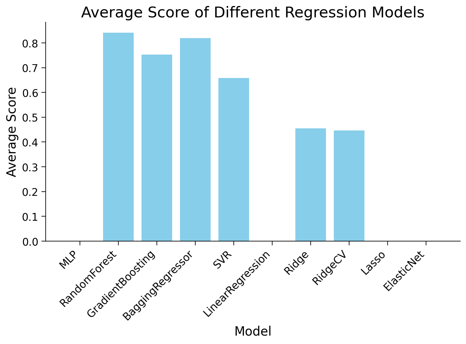
This quick sweep of models suggests Random Forest is a good choice, but recall that most of these models have hyperparameters. Varying these hyperparameters may lead to different results!
Summary#
In this tutorial, we explored how machine learning models adapt to unfamiliar emissions scenarios. Evaluating model performance on datasets representing different emission scenarios provided insights into the models’ capabilities in predicting climate variables under diverse environmental conditions.