![]()

Tutorial Objectives#
In this tutorial, you will learn about Integrated Assessment Models (IAMs), a class of models that combine climatology, economics, and social science, reflecting the intertwined nature of these domains in addressing climate change. Based on these models the IPCC established the socioeconomic pathway framework. You are going to learn how these pathways differ from one another in both climate and socioeconomic variables as well as assumptions.
After finishing this tutorial, you will know how to
filter data series of interest from a rich
pandasdata frame that contains various variables for different SSPs,tell what the abbreviation SPA stands for,
explain the differences and similarities of the SSP1-26 and SSP5-85, and
sketch the modeling approach of IAMs.
Setup#
# installations ( uncomment and run this cell ONLY when using google colab or kaggle )
# imports
import warnings
warnings.simplefilter(action='ignore', category=FutureWarning)
import seaborn as sns
import matplotlib.pyplot as plt
import pandas as pd
import numpy as np
import pooch
import os
import tempfile
Figure settings#
Show code cell source
# @title Figure settings
import ipywidgets as widgets  # interactive display

plt.style.use(
    "https://raw.githubusercontent.com/neuromatch/climate-course-content/main/cma.mplstyle"
)
Helper functions#
Show code cell source
# @title Helper functions

def pooch_load(filelocation=None, filename=None, processor=None):
    shared_location = "/home/jovyan/shared/Data/tutorials/W2D3_FutureClimate-IPCCII&IIISocio-EconomicBasis"  # this is different for each day
    user_temp_cache = tempfile.gettempdir()

    if os.path.exists(os.path.join(shared_location, filename)):
        file = os.path.join(shared_location, filename)
    else:
        file = pooch.retrieve(
            filelocation,
            known_hash=None,
            fname=os.path.join(user_temp_cache, filename),
            processor=processor,
        )

    return file


def legend_without_duplicate_labels(ax):
    handles, labels = ax.get_legend_handles_labels()
    unique = [(h, l) for i, (h, l) in enumerate(zip(handles, labels)) if l not in labels[:i]]
    ax.legend(*zip(*unique))
Section 1: Shared Socio-economic Pathways#
In this, and subsequent, tutorials, you will explore Integrated Assessment Models (IAMs) which are the standard class of models used to make climate change projections. IAMs couple a climate model with an economic model, allowing us to evaluate the two-way coupling between economic productivity and climate change severity. IAMs can also account for changes that result from mitigation efforts, which lessen anthropogenic emissions.
Let’s start by investigating some IAM model output.
The simulations are labeled by both the Shared Socioeconomic Pathway (SSP1, SSP2, SSP3, SSP4, and SSP5) and the forcing level (greenhouse gas forcing of 2.6, 7.0, 8.5 W/m2 etc. by 2100). The 5 SSPS are:
SSP1: Sustainability (Taking the Green Road)
SSP2: Middle of the Road
SSP3: Regional Rivalry (A Rocky Road)
SSP4: Inequality (A Road divided)
SSP5: Fossil-fueled Development (Taking the Highway)
We select two SSPs to exemplify how these scenarios differ from each other. To get a strong contrast, we select SSP1 and SSP5.
Let’s load the data and describe their features along a few plots.
Like in other tutorials, we provide a .csv file that is stored in the cloud and was downloaded beforehand from this IIASA database, where all data from the main simulations of the IAMs used in the IPCC reports is freely available.
# Load SSP data from .csv file
filename_SSPs = 'SSP_IAM_V2_201811.csv'
link_id = "2uwr4"
url_SSPs = f"https://osf.io/download/{link_id}/"

df = pd.read_csv(pooch_load(url_SSPs, filename_SSPs))
# get a summary of the resulting pandas dataframe
df.info()
Downloading data from 'https://osf.io/download/2uwr4/' to file '/tmp/SSP_IAM_V2_201811.csv'.
SHA256 hash of downloaded file: ec5b7bb804e49cf964d1028a7450cce96e6dd25f1ac9381326b2309063a93909
Use this value as the 'known_hash' argument of 'pooch.retrieve' to ensure that the file hasn't changed if it is downloaded again in the future.
<class 'pandas.core.frame.DataFrame'>
RangeIndex: 84353 entries, 0 to 84352
Data columns (total 16 columns):
 #   Column    Non-Null Count  Dtype
---  ------    --------------  -----
 0   MODEL     84353 non-null  object
 1   SCENARIO  84353 non-null  object
 2   REGION    84353 non-null  object
 3   VARIABLE  84353 non-null  object
 4   UNIT      84353 non-null  object
 5   2005      67962 non-null  float64
 6   2010      83666 non-null  float64
 7   2020      84227 non-null  float64
 8   2030      84227 non-null  float64
 9   2040      84227 non-null  float64
 10  2050      84224 non-null  float64
 11  2060      84224 non-null  float64
 12  2070      84224 non-null  float64
 13  2080      84215 non-null  float64
 14  2090      84215 non-null  float64
 15  2100      84215 non-null  float64
dtypes: float64(11), object(5)
memory usage: 10.3+ MB
We further explore our data frame by printing categories that are used to tag the numeric data.
print(df.SCENARIO.unique())      # print all scenarios
print(df.VARIABLE.unique()[:10]) # print the first 10 variables
print(df.REGION.unique())        # print all regions
print(df.MODEL.unique())         # print all IAMs
print(df.UNIT.unique())          # print all units
['SSP1-19' 'SSP1-26' 'SSP1-34' 'SSP1-45' 'SSP1-Baseline' 'SSP2-19'
 'SSP2-26' 'SSP2-34' 'SSP2-45' 'SSP2-60' 'SSP2-Baseline' 'SSP3-34'
 'SSP3-45' 'SSP3-60' 'SSP3-Baseline' 'SSP4-26' 'SSP4-34' 'SSP4-45'
 'SSP4-Baseline' 'SSP5-26' 'SSP5-34' 'SSP5-45' 'SSP5-60' 'SSP5-Baseline'
 'SSP4-60' 'SSP5-19' 'SSP1-60' 'SSP4-19']
['Agricultural Demand|Crops' 'Agricultural Demand|Crops|Energy'
 'Agricultural Demand|Livestock' 'Agricultural Production|Crops|Energy'
 'Agricultural Production|Crops|Non-Energy'
 'Agricultural Production|Livestock' 'Capacity|Electricity'
 'Capacity|Electricity|Biomass' 'Capacity|Electricity|Coal'
 'Capacity|Electricity|Gas']
['R5.2ASIA' 'R5.2LAM' 'R5.2MAF' 'R5.2OECD' 'R5.2REF' 'World']
['AIM/CGE' 'GCAM4' 'IMAGE' 'MESSAGE-GLOBIOM' 'REMIND-MAGPIE'
 'WITCH-GLOBIOM']
['million t DM/yr' 'GW' 'billion US$2005/yr' 'Mt BC/yr' 'Mt CH4/yr'
 'Mt CO/yr' 'Mt CO2/yr' 'Mt CO2-equiv/yr' 'kt N2O/yr' 'Mt NH3/yr'
 'Mt NO2/yr' 'Mt OC/yr' 'Mt SO2/yr' 'Mt VOC/yr' 'EJ/yr' 'million ha'
 'million' 'US$2005/t CO2' 'ppb' 'ppm' 'W/m2' '°C' 'bn tkm/yr' 'bn pkm/yr']
This file contains much data we are not interested in at the moment. To filter our example scenarios, region, and variables, we use the convenient .query() method from pandas. The VARIABLEs of interest are those we already touched on in Tutorials 1 to 3:
economic growth (
'GDP|PPP'),energy use (
'Primary Energy'),emissions (
'Emissions|Kyoto Gases'),and forcing (
'Diagnostics|MAGICC6|Forcing').As a
REGION, we choose the'World',and our
SCENARIOs are called'SSP1-26'and'SSP5-85'.The model of choice for the former scenario is by convention
'IMAGE'and'REMIND-MAGPIE'for the latter, respectively.
A function named get_SSPs_for_variable() applies all this generally and is hidden in the next cell. Please execute it, such that the subsequent cells can make use of it. If you are interested in its procedure and want to adjust it, don’t forget to save a copy beforehand.
Execute this cell to enable the dataframe filter function: get_SSPs_for_variable
Show code cell source
# @markdown *Execute this cell to enable the dataframe filter function: `get_SSPs_for_variable`*

def get_SSPs_for_variable(df,scenario,variable,region='World'):
    '''

    Function that filters IIASA's SSP database that is stored in a data frame 'df'
    and was loaded before from the 'SSP_IAM_V2_201811.csv' file.
    It returns a data frame with selected columns depending on scenario, variable and region input.
    For a given SSP scenario it chooses the conventional model for the respective scenario
    (cf. https://tntcat.iiasa.ac.at/SspDb/dsd?Action=htmlpage&page=about#v2).

    Args:
        scenario: string in "SSPX-XX" with X=1,...,5
        variable: string in df.VARIABLE, e.g. 'Population' or 'GDP|PPP'

    Returns:
        SSP data for selected columns for a given SSP scenario

    Example:
        dd = get_SSPs_for_variable(df,'SSP1-26','Population')

    '''
    ssp_model_conv = {"SSP1-Baseline" : "IMAGE",
                      "SSP1-26" : "IMAGE",
                      "SSP2-Baseline" : "MESSAGE-GLOBIOM",
                      "SSP3-Baseline" : "AIM/CGE",
                      "SSP4-Baseline" : "GCAM4",
                      "SSP5-Baseline" : "REMIND-MAGPIE"}
    model = ssp_model_conv[scenario]
    ds = df.query(
    f'(VARIABLE == "{variable}") & (SCENARIO == "{scenario}")  & (MODEL == "{model}") & (REGION == "{region}")'
)
    return ds
Let’s plot our variables of interest and compare the respective features of the scenarios.
# put variables of interest in a list
vars = ['GDP|PPP','Emissions|Kyoto Gases', 'Primary Energy','Diagnostics|MAGICC6|Forcing']
# create new names for structured data series and axes labels
val_name = ['GDP (billion US$/yr)', 'Emissions (Mt CO$_2$/yr)',  'Energy use (EJ/yr)', 'Forcing (W/m$^2$)']
# choose scenarios of interest and a color for plotting
scenarios = ['SSP1-26', 'SSP5-Baseline']
colors = ['darkblue','darkorange']

# init figure and axis
fig, axs = plt.subplots(2,2)
# loop over all variables and new names
for var, val, ax in zip(vars,val_name, axs.flatten()):

    # loop over scenarios and their color
    for sc, col in zip(scenarios, colors):
        # retrieve SSP for the respective variable from rich data frame
        ds_unstrct = get_SSPs_for_variable(df,sc,var)
        # restructure dataframe for plotting
        ds_strct = pd.melt(ds_unstrct, id_vars=["MODEL"], value_vars=['2010','2020','2030','2040','2050','2060','2070','2080','2090','2100'], var_name="YEAR", value_name =val)
        #print(ds_strct)
        # plot variable vs. time, add label incl. scenario and model
        ax.plot(ds_strct['YEAR'],ds_strct[val],label=f'{sc},\n{ds_strct.MODEL[0]}', color=col)
        # altern. plotting procedure w/o the color distinction
        #sns.lineplot(ds_strct, x='YEAR', y=val, hue='MODEL', ax=ax, palette='flare')

    # aesthetics
    ax.set_ylabel(fr'{val}')
    ax.set_xlabel('Time (years)')
    plt.setp(ax.get_xticklabels(), rotation=45)
    plt.setp(ax.get_xticklabels()[::2], visible=False)
    ax.grid(True)
    axs[0,0].legend()
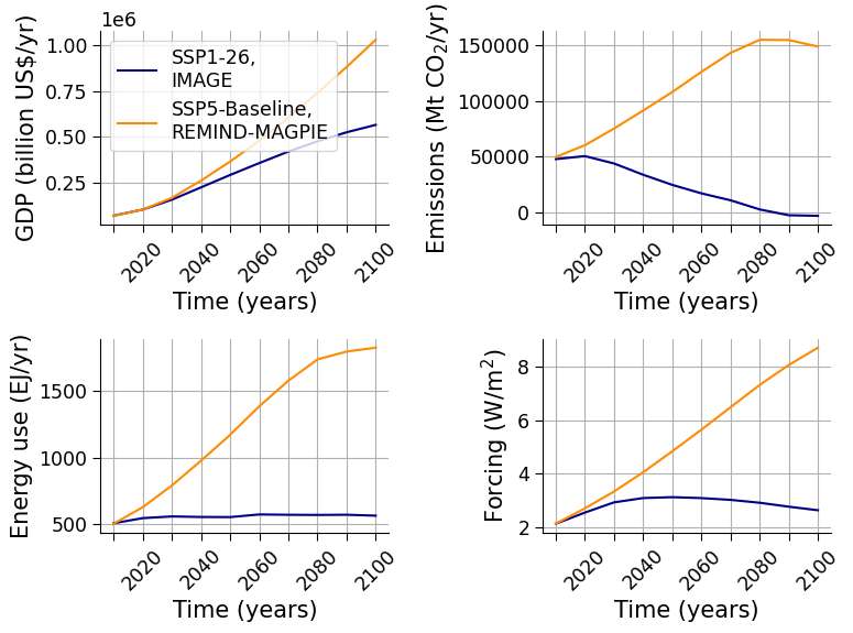
The projections in the plots you just created show changes in GDP (billion US$/yr), fossil fuel emissions (Mt CO\(_2\)/yr), energy use (EJ/yr), and forcing (W/m\(^2\)) across the two very different scenarios SSP1 and SSP5, computed at their baseline forcing level, which are each represented by a distinct color in each plot.
Our plots show that the SSP5-Baseline scenario exhibits very high levels of energy use, and emissions (due to fossil fuel exploitation), it marks the upper end of the scenarios in several dimensions (cf. Kriegler et al. (2014)).
The SSP1-26 scenario contrarily caps the increase of energy use by 2030, combined with other actions leading to decreasing emissions and subsequently a decreasing forcing for the second half of the century. However, economic growth continues with half the slope of SSP5-Baseline. In summary, it is the most optimistic projection: we transition to a global society of sustainability-focused growth.
Section 1.1: SSP Creation via IAMs#
The underlying modeling of Integrated Assessment Models (IAMs) works roughly as follows:
All SSP projections are created by optimizing economic activity within the constraint of a given level of greenhouse gas forcing at 2100 (bottom right in the above plot). This activity drives distinct temperature changes via the emissions it produces (top right), which are inputted into a damage function to compute economic damages. These damages feedback into the economy model to limit emissions-producing economic activity (top left). Note that we already explored these damage functions along our En-ROADS climate solution simulator in Tutorial 2.
The forcing constraint ensures the amount of emissions produced is consistent for that particular scenario. In other words, the projected temperature change under different scenarios is fed to a socioeconomic model component in order to assess the socioeconomic impacts resulting from the temperature change associated with each SSP. For examples of such impacts check out today’s Tutorial 2 and W2D4.
Not every variable in IAMs is endogenous (i.e. determined by other variables in the model). Some variables, like population or technology growth, are exogenous (i.e. variables whose time course is given to the model). In this case, the time course of, e.g., population and economic growth, are derived from simple growth models. These exogenous variables are assumed to be under our society’s control (e.g. via mitigation).
To understand how our plotted scenarios compare with all other scenarios, we first have a look at the underlying policy assumptions.
Section 1.3: Similarities of SSP1 and SSP5#
When you compare the two scenarios, in particular, the evolution of the population and the GDP shows how similar these scenarios are in their optimistic view on the development of humanity. We all learn to get along, both within and across countries and more equal development naturally stems from population growth through well-known mechanisms like access to conception. The following figure emphasizes this.
# put variables of interest in a list
vars = ['Population', 'GDP|PPP']
# create new names for structured data series and plot labels
val_name = ['Population\n(millions)', 'GDP (billion US$/yr)']
# choose scenarios of interest and a color for plotting
scenarios = ['SSP1-26', 'SSP5-Baseline']
colors = ['darkblue','darkorange']

# init figure and axis
fig, axs = plt.subplots(2,1)
# loop over all variables and new names
for var, val, ax in zip(vars,val_name, axs.flatten()):

    # loop over scenarios and their color
    for sc, col in zip(scenarios, colors):
        # retrieve SSP for the respective variable from rich dataframe
        ds_unstrct = get_SSPs_for_variable(df,sc,var)
        # restructure dataframe for plotting
        ds_strct = pd.melt(ds_unstrct, id_vars=["MODEL"], value_vars=['2010','2020','2030','2040','2050','2060','2070','2080','2090','2100'], var_name="YEAR", value_name =val)
        #print(ds_strct)
        # plot variable vs. time, add label incl. scenario and model
        ax.plot(ds_strct['YEAR'],ds_strct[val],label=f'{sc},\n{ds_strct.MODEL[0]}', color=col)
        # altern. plotting procedure w/o the color distinction
        #sns.lineplot(ds_strct, x='YEAR', y=val, hue='MODEL', ax=ax, palette='flare')

    # aesthetics
    ax.set_ylabel(fr'{val}')
    ax.set_xlabel('Time (years)')
    plt.setp(ax.get_xticklabels(), rotation=45)
    plt.setp(ax.get_xticklabels()[::2], visible=False)
    ax.grid(True)
    axs[0].legend()
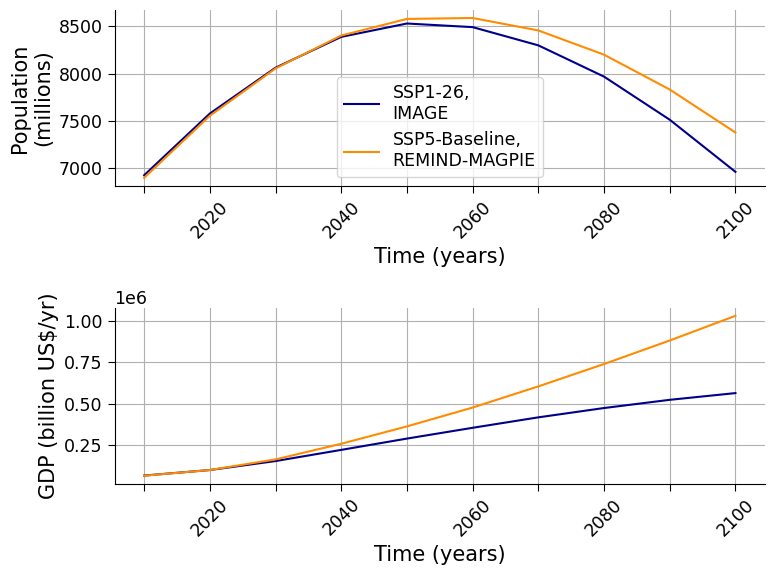
Both GDP and population increase.
Section 1.3: Differences of SSP1 and SSP5#
Major differences are visible when you contrast emissions and assume direct causation with ecosystem health. Increasing emissions then translate into decreasing ecosystem health.
Coding exercise 1.3#
Choose two variables to emphasize ecosystem health differences in the SSP1 and SSP5 scenarios and assign them to
vars. Then assign axis labels with the correct units for plotting to theval_namevariable.Explain to your pod why the chosen variables emphasize a difference in the scenarios and describe this difference based on your current knowledge of the narratives.
# put two variables of interest in a list
vars = ...
# create new names for structured data series and plot labels
val_name = ...
# choose scenarios of interest and a color for plotting
scenarios = ['SSP1-26', 'SSP5-Baseline']
colors = ['darkblue','darkorange']

#################################################
## TODO for students:
## Put two variables of interest in a list and assign it to 'vars'.
## Create new names for the structured data series and axes labels,
## put them in a list and assign it to 'val_name'.
## Remove the following line of code once you have completed the exercise:
raise NotImplementedError("Student exercise: Put two variables of interest in a list and assign it to vars. Create new names for the structured data series and axes labels, put them in a list and assign it to val_name.")
#################################################

# init figure and axis
fig, axs = plt.subplots(2,1)
# loop over all variables and new names
for var, val, ax in zip(vars,val_name, axs.flatten()):

    # loop over scenarios and their color
    for sc, col in zip(scenarios, colors):
        # retrieve SSP for the respective variable from rich dataframe
        ds_unstrct = get_SSPs_for_variable(df,sc,var)
        # restructure dataframe for plotting
        ds_strct = pd.melt(ds_unstrct, id_vars=["MODEL"], value_vars=['2010','2020','2030','2040','2050','2060','2070','2080','2090','2100'], var_name="YEAR", value_name =val)
        #print(ds_strct)
        # plot variable vs. time, add label incl. scenario and model
        ax.plot(ds_strct['YEAR'],ds_strct[val],label=f'{sc},\n{ds_strct.MODEL[0]}', color=col)
        # altern. plotting procedure w/o the color distinction
        #sns.lineplot(ds_strct, x='YEAR', y=val, hue='MODEL', ax=ax, palette='flare')

    # aesthetics
    ax.set_ylabel(fr'{val}')
    ax.set_xlabel('Time (years)')
    plt.setp(ax.get_xticklabels(), rotation=45)
    plt.setp(ax.get_xticklabels()[::2], visible=False)
    ax.grid(True)
    axs[0].legend()
Example output:

Summary#
In this tutorial, you’ve gained a first understanding of the Shared Socioeconomic Pathways and their creation, the application of Integrated Assessment Models in climate economics. You’ve learned how SSPs share policy assumptions. Furthermore, you compared SSP1 and SSP5 with respect to their view on the development of humanity and their ecosystem health.
In the next tutorial, you dissect and analyze the SSP narratives in more detail.
Resources#
It is possible to download the SSP data used in this tutorial, when you provide an email address, from this IIASA database, where all data from the main simulations of the IAMs used in the IPCC reports is freely available.
Find a summary of all SSP narratives in this paper by Oneill et al. (2017).
Find even more information in