Bonus Tutorial 7: Non-Stationarity in the EVT-framework

Bonus Tutorial 7: Non-Stationarity in the EVT-framework#

Week 2, Day 4, Extremes & Variability

Content creators: Matthias Aengenheyster, Joeri Reinders

Content reviewers: Younkap Nina Duplex, Sloane Garelick, Paul Heubel, Zahra Khodakaramimaghsoud, Peter Ohue, Laura Paccini, Jenna Pearson, Agustina Pesce, Derick Temfack, Peizhen Yang, Cheng Zhang, Chi Zhang, Ohad Zivan

Content editors: Paul Heubel, Jenna Pearson, Chi Zhang, Ohad Zivan

Production editors: Wesley Banfield, Paul Heubel, Jenna Pearson, Konstantine Tsafatinos, Chi Zhang, Ohad Zivan

Our 2024 Sponsors: CMIP, NFDI4Earth

Tutorial Objectives#

Estimated timing of tutorial: 30 minutes

In this tutorial, we will enhance our GEV model by incorporating non-stationarity to achieve a better fit for the sea surface height data from Washington DC we analyzed previously.

By the end of the tutorial you will be able to:

Apply a GEV distribution to a non-stationary record by including a time-dependent parameter.
Compare and analyze the fits of various models with different time-dependent parameters (e.g., location, scale, or shape).
Calculate effective return levels using our non-stationary GEV model.

Setup#

# installations ( uncomment and run this cell ONLY when using google colab or kaggle )

# !pip install -q condacolab
# import condacolab
# condacolab.install()
# !mamba install eigen numpy matplotlib seaborn pandas cartopy scipy texttable intake xarrayutils xmip cf_xarray intake-esm
# !pip install https://github.com/yrobink/SDFC-python/archive/master.zip

# # get some accessory functions (you will need to install wget)
!wget https://raw.githubusercontent.com/neuromatch/climate-course-content/main/tutorials/W2D4_ClimateResponse-Extremes%26Variability/extremes_functions.py
!wget https://raw.githubusercontent.com/neuromatch/climate-course-content/main/tutorials/W2D4_ClimateResponse-Extremes%26Variability/gev_functions.py
!wget https://raw.githubusercontent.com/neuromatch/climate-course-content/main/tutorials/W2D4_ClimateResponse-Extremes%26Variability/sdfc_classes.py

--2024-06-20 22:45:04--  https://raw.githubusercontent.com/neuromatch/climate-course-content/main/tutorials/W2D4_ClimateResponse-Extremes%26Variability/extremes_functions.py
Resolving raw.githubusercontent.com (raw.githubusercontent.com)... 185.199.111.133, 185.199.108.133, 185.199.109.133, ...
Connecting to raw.githubusercontent.com (raw.githubusercontent.com)|185.199.111.133|:443... connected.
HTTP request sent, awaiting response... 

200 OK
Length: 16040 (16K) [text/plain]
Saving to: ‘extremes_functions.py.1’


extremes_functions.   0%[                    ]       0  --.-KB/s               
extremes_functions. 100%[===================>]  15.66K  --.-KB/s    in 0s      

2024-06-20 22:45:04 (93.8 MB/s) - ‘extremes_functions.py.1’ saved [16040/16040]

--2024-06-20 22:45:04--  https://raw.githubusercontent.com/neuromatch/climate-course-content/main/tutorials/W2D4_ClimateResponse-Extremes%26Variability/gev_functions.py
Resolving raw.githubusercontent.com (raw.githubusercontent.com)... 185.199.109.133, 185.199.110.133, 185.199.111.133, ...
Connecting to raw.githubusercontent.com (raw.githubusercontent.com)|185.199.109.133|:443... connected.
HTTP request sent, awaiting response... 

200 OK
Length: 3739 (3.7K) [text/plain]
Saving to: ‘gev_functions.py.1’


gev_functions.py.1    0%[                    ]       0  --.-KB/s               
gev_functions.py.1  100%[===================>]   3.65K  --.-KB/s    in 0s      

2024-06-20 22:45:04 (58.7 MB/s) - ‘gev_functions.py.1’ saved [3739/3739]

--2024-06-20 22:45:05--  https://raw.githubusercontent.com/neuromatch/climate-course-content/main/tutorials/W2D4_ClimateResponse-Extremes%26Variability/sdfc_classes.py
Resolving raw.githubusercontent.com (raw.githubusercontent.com)... 185.199.108.133, 185.199.110.133, 185.199.111.133, ...
Connecting to raw.githubusercontent.com (raw.githubusercontent.com)|185.199.108.133|:443... connected.
HTTP request sent, awaiting response... 

200 OK
Length: 31925 (31K) [text/plain]
Saving to: ‘sdfc_classes.py’


sdfc_classes.py       0%[                    ]       0  --.-KB/s               
sdfc_classes.py     100%[===================>]  31.18K  --.-KB/s    in 0s      

2024-06-20 22:45:05 (88.5 MB/s) - ‘sdfc_classes.py’ saved [31925/31925]

# imports
import numpy as np
import matplotlib.pyplot as plt
import seaborn as sns
import pandas as pd
from scipy import stats
from scipy.stats import genextreme as gev
import pooch
import os
import tempfile
import gev_functions as gf
import extremes_functions as ef
import sdfc_classes as sd

---------------------------------------------------------------------------
ModuleNotFoundError                       Traceback (most recent call last)
Cell In[2], line 12
     10 import tempfile
     11 import gev_functions as gf
---> 12 import extremes_functions as ef
     13 import sdfc_classes as sd

File ~/work/climate-course-content/climate-course-content/tutorials/W2D4_ClimateResponse-Extremes&Variability/student/extremes_functions.py:2
      1 import numpy as np
----> 2 import SDFC as sd
      3 import xarray as xr
      4 import matplotlib.pyplot as plt

ModuleNotFoundError: No module named 'SDFC'

Figure Settings#

Helper functions#

Video 1: Non-Stationarity and EVT#

Section 0: Definitions and Concepts from Previous Tutorials#

Glossary widget#

Section 1: Download and Explore the Data#

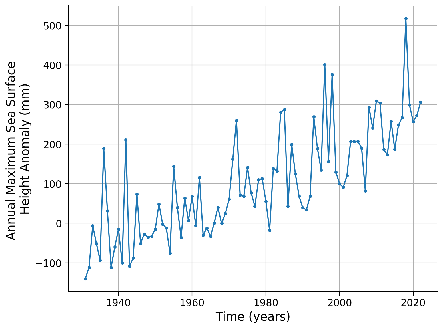
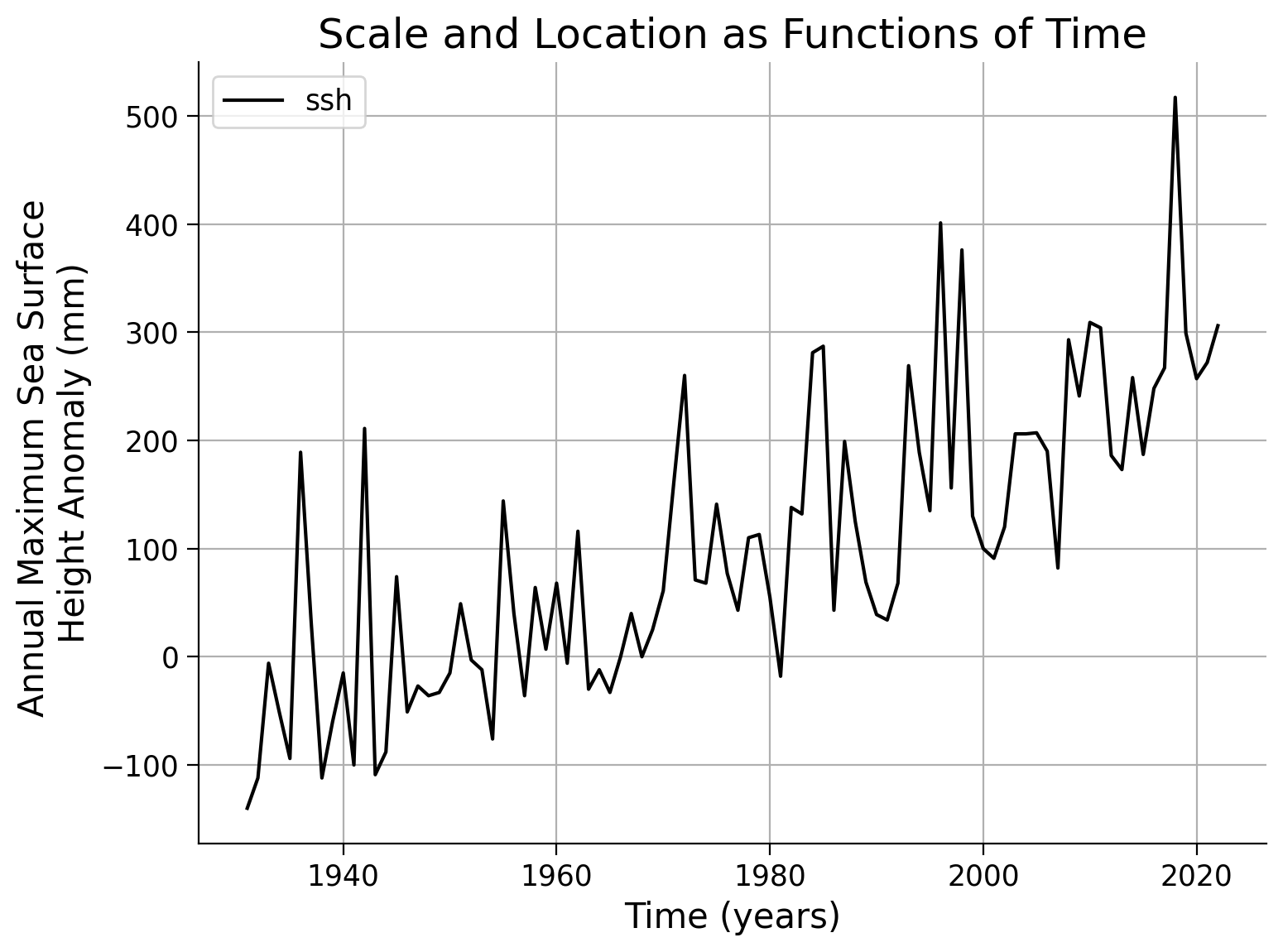
As before, we start by visually inspecting the data. Create a plot of the recorded data over time.

# download file: 'WashingtonDCSSH1930-2022.csv'
filename_WashingtonDCSSH1 = "WashingtonDCSSH1930-2022.csv"
url_WashingtonDCSSH1 = "https://osf.io/4zynp/download"
data = pd.read_csv(
    pooch_load(url_WashingtonDCSSH1, filename_WashingtonDCSSH1), index_col=0
).set_index("years")

data.ssh.plot(
    linestyle="-",
    marker=".",
    ylabel="Annual Maximum Sea Surface \nHeight Anomaly (mm)",
    xlabel="Time (years)",
    grid=True
)

<Axes: xlabel='Time (years)', ylabel='Annual Maximum Sea Surface \nHeight Anomaly (mm)'>

../../../_images/7a77f386a012c7a8e8908dcdba064cbbe7ae5b353c85ac72079ac5e34f8fba1c.png

As before, we fit a stationary Generalized Extreme Value (GEV) distribution to the data and print the resulting fit parameters:

# fit once
shape, loc, scale = gev.fit(data.ssh.values, 0)
print(f"Fitted parameters:\nLocation: {loc:.5f}, Scale: {scale:.5f}, Shape: {shape:.5f}\n")

# bootstrap approach with 100 repetitions (N_boot) to quantify uncertainty range
fit = gf.fit_return_levels(data.ssh.values, years=np.arange(1.1, 1000), N_boot=100)

Fitted parameters:
Location: 45.24719, Scale: 117.00894, Shape: 0.11541

Location: 4.5e+01, scale: 1.2e+02, shape: 1.2e-01

Ranges with alpha=0.050 :
Location: [18.62 , 72.70]
Scale: [101.10 , 133.50]
Shape: [-0.00 , 0.32]

The former gev.fit() is also implemented in the fit_return_levels() function from our helper script gev_functions.py, hence this resulted in similar parameter estimates. The latter list shows the resulting ranges of the bootstrap approach that helps to quantify the uncertainty range.

The following figure integrates multiple elements, including the QQ-plot (as discussed in previous tutorials), the comparison between modeled and empirical probability density functions, and the fitted return level plot as well as the uncertainty estimate from the bootstrapping approach.

# create figures
fig, axs = plt.subplots(2, 2, constrained_layout=True)
# reduce dimension of axes to have only one index
ax = axs.flatten()


# create x-data for QQ-plot (top left)
x = np.linspace(0, 1, 100)

# calculate quantiles by sorting from min to max
# and plot vs. return levels calculated with ppf (percent point function) and GEV fit parameters,
# cf. e.g. Tut4)
ax[0].plot(gev.ppf(x, shape, loc=loc, scale=scale), np.quantile(data.ssh, x), "o")

# plot identity line
xlim = ax[0].get_xlim()
ylim = ax[0].get_ylim()
ax[0].plot(
    [min(xlim[0], ylim[0]), max(xlim[1], ylim[1])],
    [min(xlim[0], ylim[0]), max(xlim[1], ylim[1])],
    "k",
)
#ax[0].set_xlim(xlim)
#ax[0].set_ylim(ylim)

# create x-data in SSH-data range for a methodology comparison (bottom left)
x = np.linspace(data.ssh.min() - 200, data.ssh.max() + 200, 1000)

# plot PDF of modeled GEV and empirical PDF estimate (kernel density estimation)
ax[2].plot(x, gev.pdf(x, shape, loc=loc, scale=scale), label="Modeled")
sns.kdeplot(data.ssh, ax=ax[2], label="Empirical")

# add legend
ax[2].legend()


# plot return levels (bottom right) using functions also used in Tutorial 6
gf.plot_return_levels(fit, ax=ax[3])
ax[3].set_xlim(1.5, 1000)
ax[3].set_ylim(0, None)

# aesthetics
ax[0].set_title("QQ-plot")
ax[2].set_title("PDF")
ax[3].set_title("Return Levels")

ax[0].set_xlabel("SSH Anomalies (mm)")
ax[0].set_ylabel("Return Levels (mm)")

ax[2].set_xlabel("SSH Anomalies (mm)")
ax[3].set_xlabel("Return Periods (years)")
ax[3].set_ylabel("Return Levels (mm)")

ax[1].remove() # remove top right axis

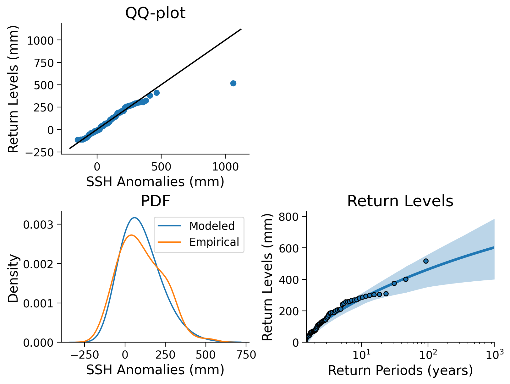
../../../_images/3690b70dfcc0420fcd1e84f2945a35ad621ebeb9b1f16d3a7f55c03ec36ab9a2.png

Click here for a detailed description of the plot.

Top left: The QQ-plot shows the quantiles versus the return levels both in millimeters, calculated from the sea surface height (SSH) anomaly data and emphasized as blue dots. For small quantiles, the return levels follow the identity line (black), in contrast to larger quantiles, where return levels increase with a smaller slope than the id line. This indicates a difference in the distributions of the two properties.

Bottom left: A comparison between modeled and empirical probability density functions (PDFs) shows different distributions. The empirical PDF weights the density of larger anomalies more heavily, so it appears that the GEV PDF underestimates large SSH anomalies. In addition, the modeled scale parameter yields a higher maximum than the empirical estimate. The tails are well comparable.

Bottom right The fitted return levels of the SSH anomalies in millimeters versus return periods log-scaled in years. Blue dots highlight the empirical calculations (using the algorithm introduced in Tutorial 2), while the blue line emphasizes the fitted GEV corresponding relationship. Shaded areas represent the uncertainty ranges that were calculated with a bootstrap approach before. The larger the return periods, the less data on such events is given, hence the uncertainty increases.

We use the function estimate_return_level_period() to compute the X-year return level:

# X-year of interest
x = 100
print(
    "{}-year return level: {:.2f} mm".format(x,
        gf.estimate_return_level_period(x, loc, scale, shape).mean()
    )
)

100-year return level: 462.88 mm

We have the option to make our GEV (Generalized Extreme Value) model non-stationary by introducing a time component to the GEV parameters. This means that the parameters will vary with time or can be dependent on other variables such as global air temperature. We call this adding covariates to parameters.

The simplest way to implement a non-stationary GEV model is by adding a linear time component to the location parameter. Instead of a fixed location parameter like “100”, it becomes a linear function of time (e.g., \(\text{time} * 1.05 + 80\)). This implies that the location parameter increases with time. We can incorporate this into our fitting process. The scipy GEV implementation does not support covariates. Therefore for this part, we will use classes and functions from the package SDFC (cf. sdfc_classes.py) and are particularly using the c_loc option - to add a covariate (c) to the location parameter (loc).

# instantiate a GEV distribution
law_ns = sd.GEV()

Due to our small data sample, our fitting method is not always converging to a non-trivial (non-zero) solution. To find adequate parameters of the GEV distribution, we therefore repeat the fitting procedure until we find non-zero coefficients (coef_).

# fit the GEV to the data, while specifying that the location parameter ('loc') is meant
# to be a covariate ('c_') of the time axis (data.index)
for i in range(250):
    law_ns.fit(data.ssh.values, c_loc=np.arange(data.index.size))
    #print(law_ns.coef_)
    # if the first coefficient is not zero, we stop fitting
    if law_ns.coef_[0] != 0:
        print(f'Found non-trivial solution after {i} fitting iterations.')
        print(law_ns.coef_)
        break

We can use a helper function named print_law() from the extreme_functions.py script to create a prettified and readable table that contains all fitted parameters.

ef.print_law(law_ns)

Now the location parameter is of type Covariate (that is, it covaries with the array we provided to c_loc), and it now consists of two coefficients (intercept and slope) of the linear relationship between the location parameter and the provided array.

As observed, we established a linear relationship by associating the location parameter with a simple array of sequential numbers (1, 2, 3, 4, 5, 6, etc.). Alternatively, if we had used an exponential function of time (e.g., 1, 2, 4, 8, 16, by setting c_loc = np.exp(np.arange(data.index.size)/data.index.size)), we would have created an exponential relationship.

Similarly, squaring the array (c_loc = np.arange(data.index.size)**2) would have resulted in a quadratic relationship. Note that our subset of SDFC classes is not tested with these exponential and squared relationships, hence a separate installation might be necessary to apply them.

It’s worth noting that various types of relationships can be employed, and this approach can be extended to multiple parameters by utilizing c_scale and c_shape. For instance, it’s possible to establish a relationship with the global mean CO₂ concentration rather than solely relying on time, which could potentially enhance the fitting accuracy.

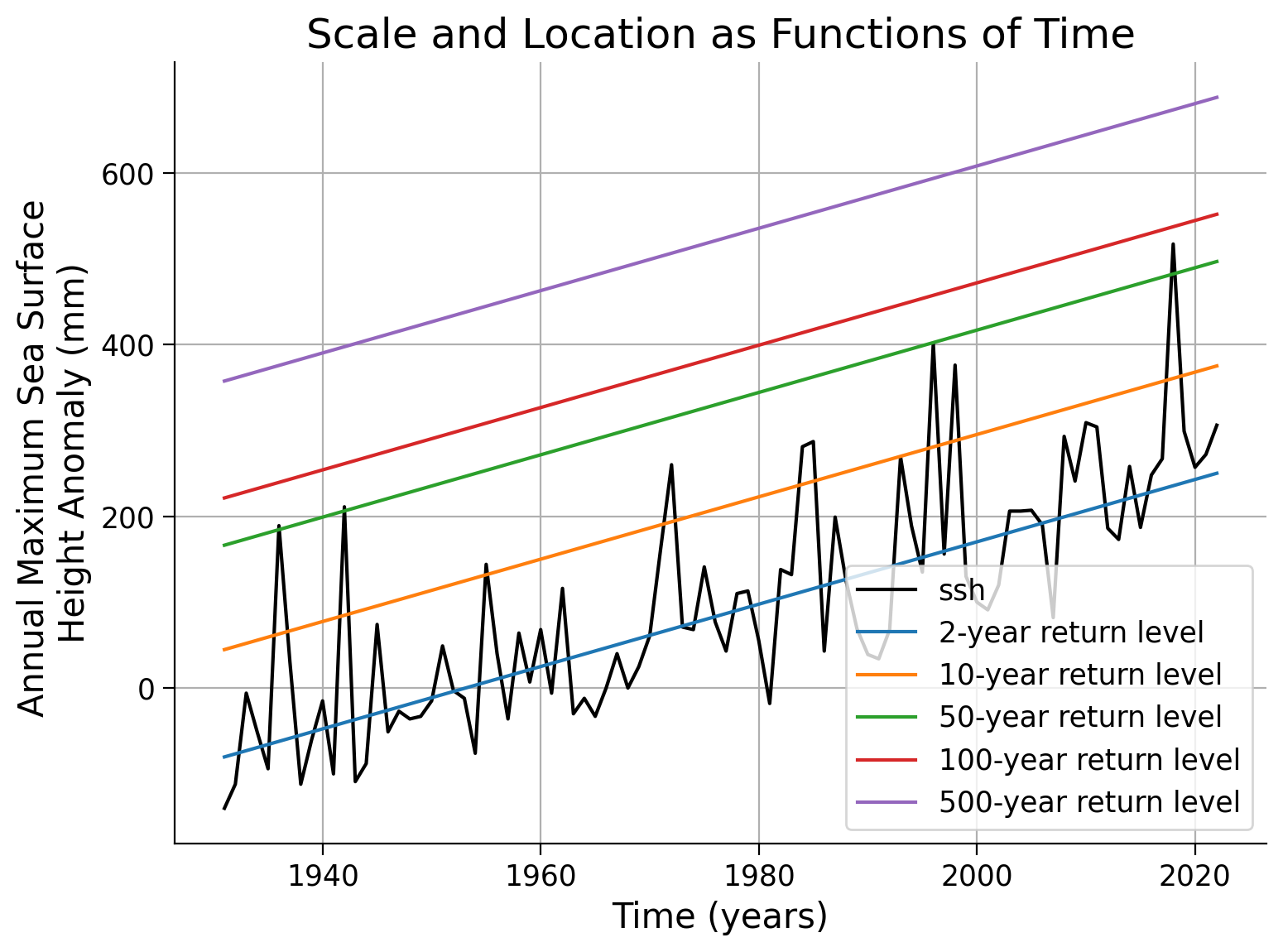
Since the location parameter is now time-dependent, we are unable to create a return level/return period plot as we did in the previous tutorials. This would require 93 separate plots, one for each year. However, there is an alternative approach that is visually appealing. We can calculate the level of the X-year event over time and overlay it onto our SSH (Sea Surface Height) anomaly record. This is referred to as the “effective return levels”.

fig, ax = plt.subplots()
# plot SSH time series
data.ssh.plot(c="k", label="sea level anomaly", ax=ax)

# years of interest
x_years = [2, 10, 50, 100, 500]

# repeat plotting of effective return levels for all years of interest
for x in x_years:
    ax.plot(
        data.index, estimate_return_level(1 - 1 / x, law_ns), label=f"{x}-year return level"
    )

ax.legend()
ax.grid(True)
ax.set_ylabel("Annual Maximum Sea Surface \nHeight Anomaly (mm)")
ax.set_xlabel("Time (years)")

You can evaluate the quality of your model fit by examining the AIC value. The Akaike Information Criterion (AIC) is useful to estimate how well the model fits the data, while preferring simpler models with fewer free parameters. A lower AIC value indicates a better fit. In the code provided below, a simple function is defined to calculate the AIC for a given fitted model.

def compute_aic(model):
    return 2 * len(model.coef_) + 2 * model.info_.mle_optim_result.fun

compute_aic(law_ns)

For comparison, let’s repeat the computation without the covariate by dropping the c_loc option. Then we can compute the AIC for the stationary model, and compare how well the model fits the data:

law_stat = sd.GEV()
law_stat.fit(data.ssh.values)

compute_aic(law_stat)

You can see that AIC is lower for the model that has the location parameter as a covariate - this suggests this model fits the data better.

Coding Exercises 1#

Scale and/or shape as a function of time

You have seen above how to make the location parameter a function of time, by providing the keyword c_loc to the fit() function.

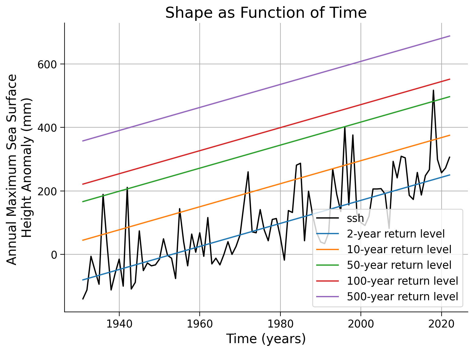
Now repeat this procedure, making scale, shape, or both parameters a function of time. To do this, you need to instantiate a new GEV object and call it e.g. law_ns_scale = sd.GEV(). Then call the .fit() function similarly to before, but replace c_loc with c_scale and/or c_shape. Plot the effective return levels by providing your fitted model to the estimate_return_level() function, as done previously. Observe if the model fits the data better, worse, or remains the same.
Lastly, compute the AIC for your new fits. Compare the AIC values to determine if the expectation from the previous step is met.

# instantiate a GEV distribution
law_ns_scale = ...

# fit the GEV to the data, while specifying that the scale parameter ('scale') is meant to be a covariate ('_c') of the time axis (data.index)
_ = ...

# plot results
fig, ax = plt.subplots()
data.ssh.plot(c="k", ax=ax)

# years of interest
x_years = [2, 10, 50, 100, 500]

# repeat plotting of effective return levels for all years of interest
for x in x_years:
    _ = ...

ax.legend()
ax.grid(True)
ax.set_xlabel("Time (years)")
ax.set_ylabel("Annual Maximum Sea Surface \nHeight Anomaly (mm)")
ax.set_title("Scale as Function of Time")

Text(0.5, 1.0, 'Scale as Function of Time')

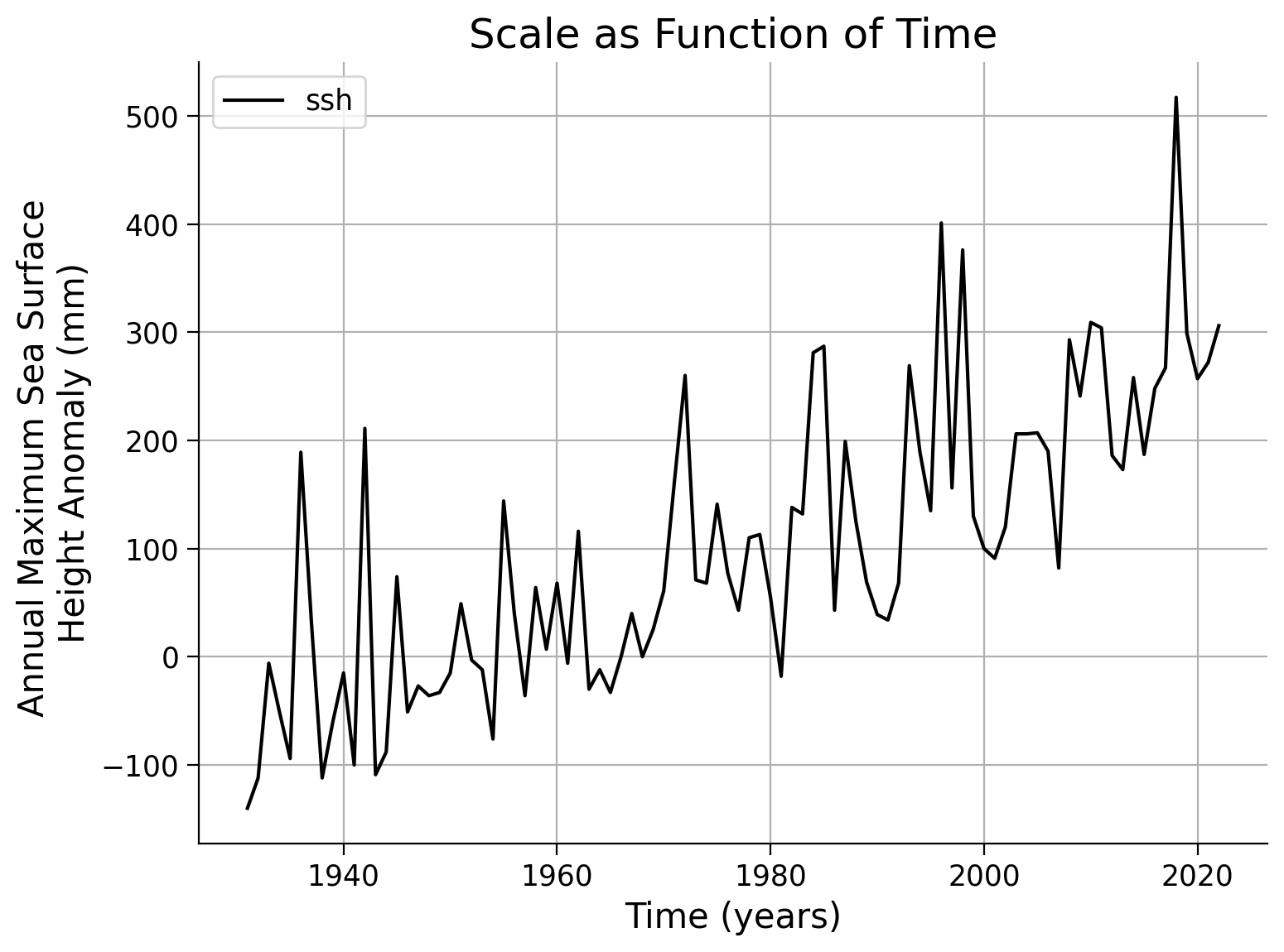
../../../_images/c03fc63dbe130535cf087d8b1ae4848adfa045bfbd861d4e9a52bea77d8cdca7.png

Click for solution

Example output:

# instantiate a GEV distribution
law_ns_shape = ...

# fit the GEV to the data, while specifying that the shape parameter ('shape') is meant to be a covariate ('_c') of the time axis (data.index)
_ = ...

# plot results
fig, ax = plt.subplots()
data.ssh.plot(c="k", ax=ax)

# years of interest
x_years = [2, 10, 50, 100, 500]

# repeat plotting of effective return levels for all years of interest
for x in x_years:
    _ = ...

ax.legend()
ax.grid(True)
ax.set_xlabel("Time (years)")
ax.set_ylabel("Annual Maximum Sea Surface \nHeight Anomaly (mm)")
ax.set_title("Shape as Function of Time")

Text(0.5, 1.0, 'Shape as Function of Time')

../../../_images/46b79172b186fe7efc70683dd63e3fb2f29f9d789bfd7c892c5820e9f704d078.png

Click for solution

Example output:

# initialize a GEV distribution
law_ns_loc_scale = ...

# fit the GEV to the data using c_loc and c_scale
_ = ...

# plot results
fig, ax = plt.subplots()
data.ssh.plot(c="k", ax=ax)

# years of interest
x_years = [2, 10, 50, 100, 500]

# repeat plotting of effective return levels for all years of interest
for x in x_years:
    _ = ...

ax.legend()
ax.grid(True)
ax.set_xlabel("Time (years)")
ax.set_ylabel("Annual Maximum Sea Surface \nHeight Anomaly (mm)")
ax.set_title("Scale and Location as Functions of Time")

Text(0.5, 1.0, 'Scale and Location as Functions of Time')

../../../_images/ca150c471ab5c6f3fcc0c936c0048f606020b43eaebf38a1d0154b4b8d19a994.png

Click for solution

Example output:

#################################################
## TODO for students:                                                                  ##
## Add the respective Akaike Information Criterion (AIC) computation to the data list. ##
# Remove or comment the following line of code once you have completed the exercise:
raise NotImplementedError("Student exercise: Add the respective Akaike Information Criterion (AIC) computation to the data list.")
#################################################

aics = pd.Series(
    index=["Location", "Scale", "Shape", "Location and Scale"],
    data=[
        ...,
        ...,
        ...,
        ...
    ],
)

aics.sort_values()

Click for solution

Summary#

In this tutorial, you adapted the GEV model to better fit non-stationary sea surface height (SSH) data from Washington DC. You learned how to:

Modify the GEV distribution to accommodate a time-dependent parameter, enabling non-stationarity.
Compare different models based on their time-dependent parameters.
Calculate effective return levels with the non-stationary GEV model.
Assessed the fit of the model using the Akaike Information Criterion (AIC).

Resources#

Original data from this tutorial can be found here. Note the data used in this tutorial were preprocessed to extract the annual maximum values.

Bonus Tutorial 7: Non-Stationarity in the EVT-framework

Contents

Bonus Tutorial 7: Non-Stationarity in the EVT-framework#

Tutorial Objectives#

Setup#

Figure Settings#

Helper functions#

Video 1: Non-Stationarity and EVT#

Section 0: Definitions and Concepts from Previous Tutorials#

Glossary widget#

Section 1: Download and Explore the Data#

Coding Exercises 1#

Summary#

Resources#