Bonus Tutorial 8: Thresholds

Bonus Tutorial 8: Thresholds#

Week 2, Day 4, Extremes & Variability

Content creators: Matthias Aengenheyster, Joeri Reinders

Content reviewers: Younkap Nina Duplex, Sloane Garelick, Paul Heubel, Zahra Khodakaramimaghsoud, Peter Ohue, Laura Paccini, Jenna Pearson, Derick Temfack, Peizhen Yang, Cheng Zhang, Chi Zhang, Ohad Zivan

Content editors: Paul Heubel, Jenna Pearson, Chi Zhang, Ohad Zivan

Production editors: Wesley Banfield, Paul Heubel, Jenna Pearson, Konstantine Tsafatinos, Chi Zhang, Ohad Zivan

Our 2024 Sponsors: CMIP, NFDI4Earth

Tutorial Objectives#

Estimated timing of tutorial: 30 minutes

The human body has physiological limits within which it can function. In hot conditions, the body cools itself through the process of sweating, where water evaporates from the skin, resulting in the loss of heat. The effectiveness of this cooling mechanism depends on the air’s capacity to hold moisture. This is why sweating is more effective in dry heat, while humid heat feels “hotter” because it hampers the body’s ability to cool down.

As a result, the combination of temperature and humidity sets limits on the body’s ability to regulate its temperature. One measure that captures this combined effect is the “wet-bulb globe temperature,” which combines information about ambient temperature, relative humidity, wind, and solar radiation to monitor heat stress risks while in direct sunlight. You can learn more about wet-bulb temperature on the following Wikipedia page: Wet-bulb globe temperature.

In this tutorial, we will look at extreme levels of wet-bulb temperature spatially and consider the importance of thresholds.

By the end of the tutorial, you will be able to:

Assess the risk of increasing wet-bulb globe temperatures.
Analyse how the probability of crossing threshold changes over time and between scenarios.
Assess the results of a spatial GEV analysis.

Setup#

# installations ( uncomment and run this cell ONLY when using google colab or kaggle )

# !pip install -q condacolab
# import condacolab
# condacolab.install()
# !mamba install numpy matplotlib seaborn pandas cartopy scipy texttable xarrayutils cf_xarray cmocean

!wget https://raw.githubusercontent.com/neuromatch/climate-course-content/main/tutorials/W2D4_ClimateResponse-Extremes%26Variability/extremes_functions.py
!wget https://raw.githubusercontent.com/neuromatch/climate-course-content/main/tutorials/W2D4_ClimateResponse-Extremes%26Variability/gev_functions.py
!wget https://raw.githubusercontent.com/neuromatch/climate-course-content/main/tutorials/W2D4_ClimateResponse-Extremes%26Variability/sdfc_classes.py

--2024-06-20 22:45:19--  https://raw.githubusercontent.com/neuromatch/climate-course-content/main/tutorials/W2D4_ClimateResponse-Extremes%26Variability/extremes_functions.py
Resolving raw.githubusercontent.com (raw.githubusercontent.com)... 185.199.111.133, 185.199.108.133, 185.199.109.133, ...
Connecting to raw.githubusercontent.com (raw.githubusercontent.com)|185.199.111.133|:443... connected.
HTTP request sent, awaiting response... 200 OK
Length: 16040 (16K) [text/plain]
Saving to: ‘extremes_functions.py.2’


extremes_functions.   0%[                    ]       0  --.-KB/s               
extremes_functions. 100%[===================>]  15.66K  --.-KB/s    in 0s      

2024-06-20 22:45:19 (102 MB/s) - ‘extremes_functions.py.2’ saved [16040/16040]

--2024-06-20 22:45:19--  https://raw.githubusercontent.com/neuromatch/climate-course-content/main/tutorials/W2D4_ClimateResponse-Extremes%26Variability/gev_functions.py
Resolving raw.githubusercontent.com (raw.githubusercontent.com)... 185.199.108.133, 185.199.109.133, 185.199.111.133, ...
Connecting to raw.githubusercontent.com (raw.githubusercontent.com)|185.199.108.133|:443... connected.
HTTP request sent, awaiting response... 200 OK
Length: 3739 (3.7K) [text/plain]
Saving to: ‘gev_functions.py.2’


gev_functions.py.2    0%[                    ]       0  --.-KB/s               
gev_functions.py.2  100%[===================>]   3.65K  --.-KB/s    in 0s      

2024-06-20 22:45:19 (56.1 MB/s) - ‘gev_functions.py.2’ saved [3739/3739]

--2024-06-20 22:45:19--  https://raw.githubusercontent.com/neuromatch/climate-course-content/main/tutorials/W2D4_ClimateResponse-Extremes%26Variability/sdfc_classes.py
Resolving raw.githubusercontent.com (raw.githubusercontent.com)... 185.199.111.133, 185.199.109.133, 185.199.108.133, ...
Connecting to raw.githubusercontent.com (raw.githubusercontent.com)|185.199.111.133|:443... connected.
HTTP request sent, awaiting response... 200 OK
Length: 31925 (31K) [text/plain]
Saving to: ‘sdfc_classes.py.1’


sdfc_classes.py.1     0%[                    ]       0  --.-KB/s               
sdfc_classes.py.1   100%[===================>]  31.18K  --.-KB/s    in 0s      

2024-06-20 22:45:19 (89.1 MB/s) - ‘sdfc_classes.py.1’ saved [31925/31925]

# imports
import xarray as xr
import matplotlib.pyplot as plt
import cartopy.crs as ccrs
import pandas as pd
import seaborn as sns
import cmocean.cm as cmo
import os
import numpy as np
from scipy import stats
from scipy.stats import genextreme as gev
import pooch
import os
import tempfile
import gev_functions as gf
import extremes_functions as ef
import sdfc_classes as sd

import warnings

warnings.filterwarnings("ignore")

---------------------------------------------------------------------------
ModuleNotFoundError                       Traceback (most recent call last)
Cell In[2], line 16
     14 import tempfile
     15 import gev_functions as gf
---> 16 import extremes_functions as ef
     17 import sdfc_classes as sd
     19 import warnings

File ~/work/climate-course-content/climate-course-content/tutorials/W2D4_ClimateResponse-Extremes&Variability/student/extremes_functions.py:2
      1 import numpy as np
----> 2 import SDFC as sd
      3 import xarray as xr
      4 import matplotlib.pyplot as plt

ModuleNotFoundError: No module named 'SDFC'

Note that import gev_functions as gf and extremes_functions as ef import the functions introduced in previous tutorials. Furthermore, import sdfc_classes as sd allows to use SDFC classes, that have been introduced in Tutorial 7.

Figure Settings#

Helper functions#

Video 1: Thresholds#

Section 1: Downloading the Data#

In this tutorial, we will utilize wet-bulb globe temperature data derived from the MPI-ESM1-2-HR climate model, developed by the Max Planck Institute for Meteorology in Hamburg, Germany. The data covers the historical period (hist) as well as three future CMIP6 climate scenarios (SSP1-2.6, SSP2-4.5, and SSP5-8.5), which were introduced on W2D1 and in the previous Tutorial 6.

You can learn more about CMIP, including the different scenarios, through our CMIP Resource Bank and the CMIP website.

During the pre-processing phase, the data was subjected to a 7-day averaging process, followed by the computation of the annual maximum. As a result, the data for each grid point represents the wet-bulb temperature during the most extreme 7-day period within each year.

# download file: 'WBGT_day_MPI-ESM1-2-HR_historical_r1i1p1f1_raw_runmean7_yearmax.nc'

filename_WBGT_day = "WBGT_day_MPI-ESM1-2-HR_historical_r1i1p1f1_raw_runmean7_yearmax.nc"
url_WBGT_day = "https://osf.io/69ms8/download"

wetbulb_hist = xr.open_dataset(pooch_load(url_WBGT_day, filename_WBGT_day)).WBGT
wetbulb_hist.attrs["units"] = "degC"

Downloading data from 'https://osf.io/69ms8/download' to file '/tmp/WBGT_day_MPI-ESM1-2-HR_historical_r1i1p1f1_raw_runmean7_yearmax.nc'.

SHA256 hash of downloaded file: 45bf7ad1aae4e282ee1ef5302bcca7becee1999e768c41c20ff96ca5526485ff
Use this value as the 'known_hash' argument of 'pooch.retrieve' to ensure that the file hasn't changed if it is downloaded again in the future.

The dataset consists of one entry per year. However, due to the inclusion of leap years, the data processing step resulted in different days assigned to each year. This discrepancy is deemed undesirable for analysis purposes. To address this, we resample the data by grouping all the data points belonging to each year and taking their average. Since there is only one data point per year, this resampling process does not alter the data itself but rather adjusts the time coordinate. This serves as a reminder to thoroughly inspect datasets before analysis, as overlooking such issues can lead to workflow failures.

wetbulb_hist = wetbulb_hist.resample(time="1Y").mean()

<string>:6: FutureWarning: 'Y' is deprecated and will be removed in a future version. Please use 'YE' instead of 'Y'.

Let’s load the data for the remaining scenarios:

# SSP1-2.6 - 'WBGT_day_MPI-ESM1-2-HR_ssp126_r1i1p1f1_raw_runmean7_yearmax.nc'
filename_SSP126 = "WBGT_day_MPI-ESM1-2-HR_ssp126_r1i1p1f1_raw_runmean7_yearmax.nc"
url_SSP126 = "https://osf.io/67b8m/download"
wetbulb_126 = xr.open_dataset(pooch_load(url_SSP126, filename_SSP126)).WBGT
wetbulb_126.attrs["units"] = "degC"
wetbulb_126 = wetbulb_126.resample(time="1Y").mean()

# SSP2-4.5 - WBGT_day_MPI-ESM1-2-HR_ssp245_r1i1p1f1_raw_runmean7_yearmax.nc
filename_SSP245 = "WBGT_day_MPI-ESM1-2-HR_ssp245_r1i1p1f1_raw_runmean7_yearmax.nc"
url_SSP245 = "https://osf.io/fsx5y/download"
wetbulb_245 = xr.open_dataset(pooch_load(url_SSP245, filename_SSP245)).WBGT
wetbulb_245.attrs["units"] = "degC"
wetbulb_245 = wetbulb_245.resample(time="1Y").mean()

# SSP5-8.5 - WBGT_day_MPI-ESM1-2-HR_ssp585_r1i1p1f1_raw_runmean7_yearmax.nc
filename_SSP585 = "WBGT_day_MPI-ESM1-2-HR_ssp585_r1i1p1f1_raw_runmean7_yearmax.nc"
url_SSP585 = "https://osf.io/pr456/download"
wetbulb_585 = xr.open_dataset(pooch_load(url_SSP585, filename_SSP585)).WBGT
wetbulb_585.attrs["units"] = "degC"
wetbulb_585 = wetbulb_585.resample(time="1Y").mean()

Downloading data from 'https://osf.io/67b8m/download' to file '/tmp/WBGT_day_MPI-ESM1-2-HR_ssp126_r1i1p1f1_raw_runmean7_yearmax.nc'.

SHA256 hash of downloaded file: 08b78a22404166a9774787a9ed4b89e452f0d28e1b15feab7f315d92eb46fbcf
Use this value as the 'known_hash' argument of 'pooch.retrieve' to ensure that the file hasn't changed if it is downloaded again in the future.

<string>:6: FutureWarning: 'Y' is deprecated and will be removed in a future version. Please use 'YE' instead of 'Y'.
Downloading data from 'https://osf.io/fsx5y/download' to file '/tmp/WBGT_day_MPI-ESM1-2-HR_ssp245_r1i1p1f1_raw_runmean7_yearmax.nc'.

SHA256 hash of downloaded file: 67a645a5447553fcc89366e74e31da28ad8852ec9e82a1b3871fe3bc7fc043c8
Use this value as the 'known_hash' argument of 'pooch.retrieve' to ensure that the file hasn't changed if it is downloaded again in the future.

<string>:6: FutureWarning: 'Y' is deprecated and will be removed in a future version. Please use 'YE' instead of 'Y'.
Downloading data from 'https://osf.io/pr456/download' to file '/tmp/WBGT_day_MPI-ESM1-2-HR_ssp585_r1i1p1f1_raw_runmean7_yearmax.nc'.

SHA256 hash of downloaded file: 8aafc51015921ed0cb76c547937db91b2077577ee9f859001d4cfa26c613bc05
Use this value as the 'known_hash' argument of 'pooch.retrieve' to ensure that the file hasn't changed if it is downloaded again in the future.

<string>:6: FutureWarning: 'Y' is deprecated and will be removed in a future version. Please use 'YE' instead of 'Y'.

Let’s look at how the data is structured:

There is one data point per year on a latitude-longitude grid. Let’s compute the grid spacing in the longitude and latitude directions:

wetbulb_hist.lon.diff("lon").values.mean()

0.9375

wetbulb_hist.lat.diff("lat").values.mean()

0.9349133773038073

Each grid box in the dataset has an approximate size of 1 degree by 1 degree, which translates to about 100 km by 100 km at the equator. However, this size decreases as we move towards the poles due to the convergence of the meridians. It is important to consider the limitations imposed by this grid resolution.

As a result, at the equator, the grid boxes cover an area of approximately 100 km by 100 km, while their size decreases in the mid-latitudes.

Considering these grid box limitations, can you identify any potential limitations or challenges they may introduce in the analysis?

Section 1.1: Focus on New Delhi, India#

Before doing spatial analysis, in the following, we focus on the capital of India: New Delhi.

# find the nearest model point to the latitude and longitude of New Delhi
wetbulb_hist_delhi = wetbulb_hist.sel(lon=77.21, lat=28.61, method="nearest")
wetbulb_126_delhi = wetbulb_126.sel(lon=77.21, lat=28.61, method="nearest")
wetbulb_245_delhi = wetbulb_245.sel(lon=77.21, lat=28.61, method="nearest")
wetbulb_585_delhi = wetbulb_585.sel(lon=77.21, lat=28.61, method="nearest")

# plot time series of all scenarios for New Delhi
fig, ax = plt.subplots()
wetbulb_hist_delhi.plot(linestyle="-", marker=".", label="hist", ax=ax)
wetbulb_126_delhi.plot(linestyle="-", marker=".", label="ssp126", ax=ax)
wetbulb_245_delhi.plot(linestyle="-", marker=".", label="ssp245", ax=ax)
wetbulb_585_delhi.plot(linestyle="-", marker=".", label="ssp585", ax=ax)

ax.legend()
ax.set_title("")
ax.set_xlabel("Time (years)")
ax.set_ylabel("Maximum 7-day Mean\nWet-Bulb Globe Temperature ($\degree$C)")
ax.grid(True)

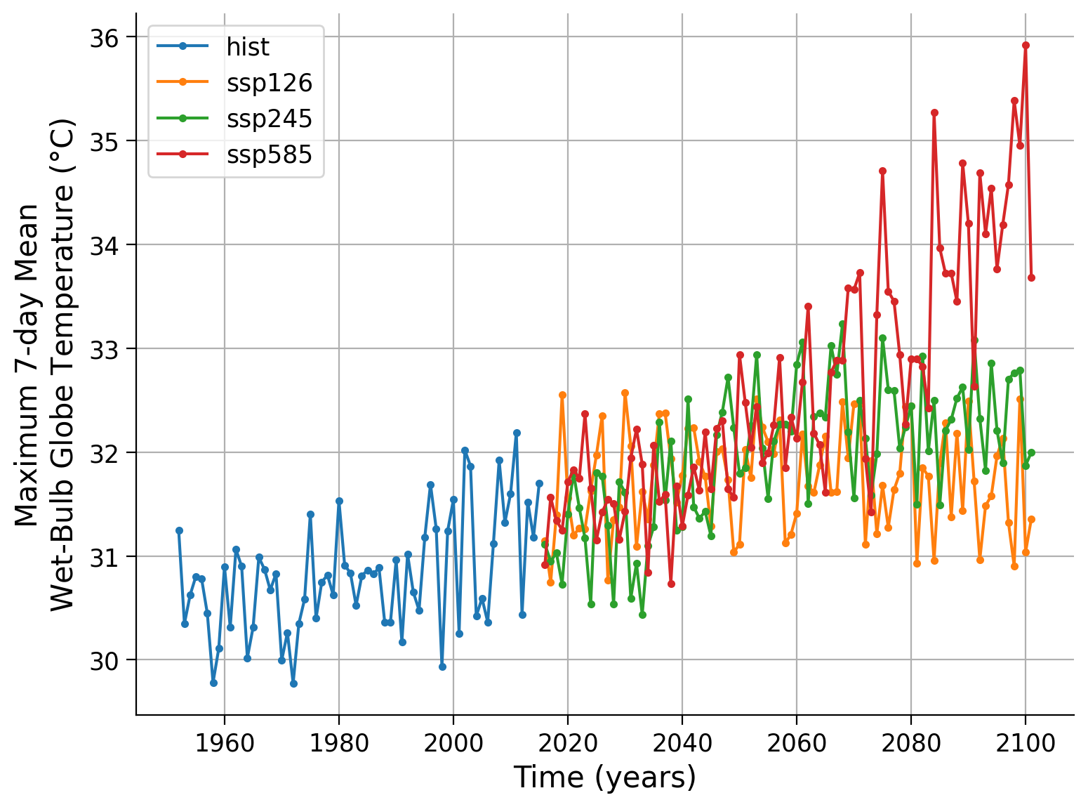
../../../_images/c58a6340d387d4cf96148129bec95d65653639765f6d70e597bb70e699cf700a.png

Note:

Trends are visible in the historical period
Distinct differences between climate scenarios are apparent
Strong variability - each years maximum is not necessarily warmer than the previous one

Let’s fit the data to a GEV distribution and get the associated return levels.

# GEV fit for historical period in New Delhi with bootstrapping for uncertainty estimation
shape_hist, loc_hist, scale_hist = gev.fit(wetbulb_hist_delhi.values, 0)
return_levels_hist = gf.fit_return_levels(
    wetbulb_hist_delhi.values, years=np.arange(1.1, 1000), N_boot=100
)

Location: 3.1e+01, scale: 5.0e-01, shape: 1.6e-01

Ranges with alpha=0.050 :
Location: [30.46 , 30.76]
Scale: [0.41 , 0.60]
Shape: [0.00 , 0.33]

Now we can plot the probability density functions, the return levels, and assess the fit using the QQ plot from previous tutorials.

# create figures
fig, axs = plt.subplots(2, 2, constrained_layout=True)
# reduce dimension of axes to have only one index
ax = axs.flatten()

# create x-data for QQ-plot (top left)
x = np.linspace(0, 1, 100)

# calculate quantiles by sorting from min to max
# and plot vs. return levels calculated with ppf (percent point function) and GEV fit parameters,
# cf. e.g. Tut4)
ax[0].plot(
    gev.ppf(x, shape_hist, loc=loc_hist, scale=scale_hist),
    np.quantile(wetbulb_hist_delhi, x),
    "o",
)
# plot identity line
xlim = ax[0].get_xlim()
ylim = ax[0].get_ylim()
ax[0].plot(
    [min(xlim[0], ylim[0]), max(xlim[1], ylim[1])],
    [min(xlim[0], ylim[0]), max(xlim[1], ylim[1])],
    "k",
)

#ax[0].set_xlim(xlim)
#ax[0].set_ylim(ylim)

# create time data array for PDF comparison (bottom left)
x = np.linspace(wetbulb_hist_delhi.min() - 1, wetbulb_hist_delhi.max() + 1, 1000)
wetbulb_hist_delhi.plot.hist(
    bins=np.arange(29, 33, 0.25),
    histtype="step",
    density=True,
    lw=1,
    color="k",
    ax=ax[2],
    label="histogram",
)
# methodology comparison (bottom left)
# plot PDF of modeled GEV and empirical PDF estimate (kernel density estimation)
ax[2].plot(x, gev.pdf(x, shape_hist, loc=loc_hist, scale=scale_hist), label="Modeled")
sns.kdeplot(wetbulb_hist_delhi, ax=ax[2], label="Empirical")
ax[2].legend()

# plot return levels (bottom right) using functions also used in Tutorial 6 and 7
gf.plot_return_levels(return_levels_hist, ax=ax[3])
ax[3].set_xlim(1.5, 1000)
# ax[3].set_ylim(0,None)

# aesthetics
ax[0].set_title("QQ-plot")
ax[2].set_title("PDF")
ax[3].set_title("Return levels")

ax[0].set_xlabel("Wet-Bulb Globe Temperature ($\degree$C)")
ax[0].set_ylabel("Return Levels ($\degree$C)")

ax[2].set_xlabel("Wet-Bulb Globe Temperature ($\degree$C)")
ax[3].set_xlabel("Return Periods (years)")
ax[3].set_ylabel("Return Levels ($\degree$C)")

ax[1].remove()

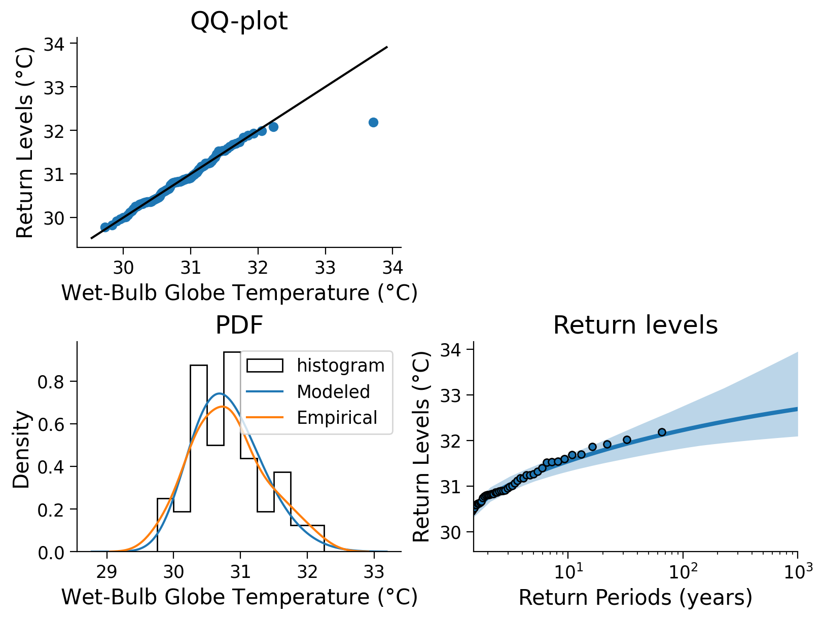
../../../_images/2724fb45ba811ae7d9f83565c3cf80a057b632339177d60c082107a61eb73eae.png

Click here for a detailed description of the plot.

Top left: The QQ-plot shows the quantiles versus the return levels both in $\degree$C, calculated from the wet-bulb globe temperature data and emphasized as blue dots. For small quantiles, the return levels follow the identity line (black), in contrast to a few larger quantiles, where return levels increase with a smaller slope than the id line. This indicates a slight difference in the distributions of the two properties.

Bottom left: A comparison between modeled and empirical probability density functions (PDFs) shows slightly different distributions. The empirical PDF weights the density of larger anomalies more, so it appears that the GEV PDF underestimates large wet-bulb globe temperatures. In addition, the modeled scale parameter yields a higher maximum than the empirical estimate. The tails are comparable, however the empirical PDF sees more events in the extremes.

Bottom right: The fitted return levels of the wet-bulb globe temperatures in $\degree$C versus return periods log-scaled in years. Blue dots highlight the empirical calculations (using the algorithm introduced in Tutorial 2), while the blue line emphasizes the fitted GEV corresponding relationship. Shaded areas represent the uncertainty ranges that were calculated with a bootstrap approach before. The larger the return periods, the less data on such events is given, hence the uncertainty increases.

We use the function estimate_return_level_period() to compute the X-year return level:

# X-year of interest
x = 100
print(
    "{}-year return level: {:.2f} C".format(x,
        gf.estimate_return_level_period(x, loc_hist, scale_hist, shape_hist).mean()
    )
)

100-year return level: 32.23 C

Now let’s compare with the last 30 years of the SSP-245 scenario, the middle scenario we looked at before. 2050-2100 are approximately stationary here, so we can leave out that utility.

shape_245, loc_245, scale_245 = gev.fit(
    wetbulb_245_delhi.sel(time=slice("2070", "2100")).values, 0
)
return_levels_245 = gf.fit_return_levels(
    wetbulb_245_delhi.sel(time=slice("2070", "2100")).values,
    years=np.arange(1.1, 1000),
    N_boot=100,
)

Location: 3.2e+01, scale: 4.5e-01, shape: 3.8e-01

Ranges with alpha=0.050 :
Location: [31.96 , 32.45]
Scale: [0.32 , 0.58]
Shape: [0.00 , 0.84]

# create figures
fig, axs = plt.subplots(2, 2, constrained_layout=True)
# reduce dimension of axes to have only one index
ax = axs.flatten()

# create x-data for QQ-plot (top left)
x = np.linspace(0, 1, 100)

# calculate quantiles by sorting from min to max
# and plot vs. return levels calculated with ppf (percent point function) and GEV fit parameters,
# cf. e.g. Tut4)
ax[0].plot(
    gev.ppf(x, shape_245, loc=loc_245, scale=scale_245),
    np.quantile(wetbulb_245_delhi.sel(time=slice("2051", "2100")), x),
    "o",
)
# plot identity line
xlim = ax[0].get_xlim()
ylim = ax[0].get_ylim()
ax[0].plot(
    [min(xlim[0], ylim[0]), max(xlim[1], ylim[1])],
    [min(xlim[0], ylim[0]), max(xlim[1], ylim[1])],
    "k",
)

#ax[0].set_xlim(xlim)
#ax[0].set_ylim(ylim)

# create time data array for PDF comparison (bottom left)
x = np.linspace(
    wetbulb_245_delhi.sel(time=slice("2051", "2100")).min() - 1,
    wetbulb_245_delhi.sel(time=slice("2051", "2100")).max() + 1,
    1000,
)
# plot histogram
wetbulb_245_delhi.sel(time=slice("2051", "2100")).plot.hist(
    bins=np.arange(29, 33, 0.25),
    histtype="step",
    density=True,
    lw=1,
    color="k",
    ax=ax[2],
    label="histogram",
)
# add GEV PDF defined by fit parameters
ax[2].plot(x, gev.pdf(x, shape_245, loc=loc_245, scale=scale_245), label="Modeled")
# add kernel density estimation (kde) of PDF
sns.kdeplot(
    wetbulb_245_delhi.sel(time=slice("2051", "2100")), ax=ax[2], label="Empirical"
)
ax[2].legend()

# plot return levels (bottom right) using functions also used in Tutorial 6 and 7
gf.plot_return_levels(return_levels_245, ax=ax[3])
ax[3].set_xlim(1.5, 1000)
# ax[3].set_ylim(0,None)

# aesthetics
ax[0].set_title("QQ-plot")
ax[2].set_title("PDF")
ax[3].set_title("Return levels")

ax[0].set_xlabel("Wet-Bulb Globe Temperature ($\degree$C)")
ax[0].set_ylabel("Return Levels ($\degree$C)")

ax[2].set_xlabel("Wet-Bulb Globe Temperature ($\degree$C)")
ax[3].set_xlabel("Return Periods (years)")
ax[3].set_ylabel("Return Levels ($\degree$C)")

ax[1].remove()

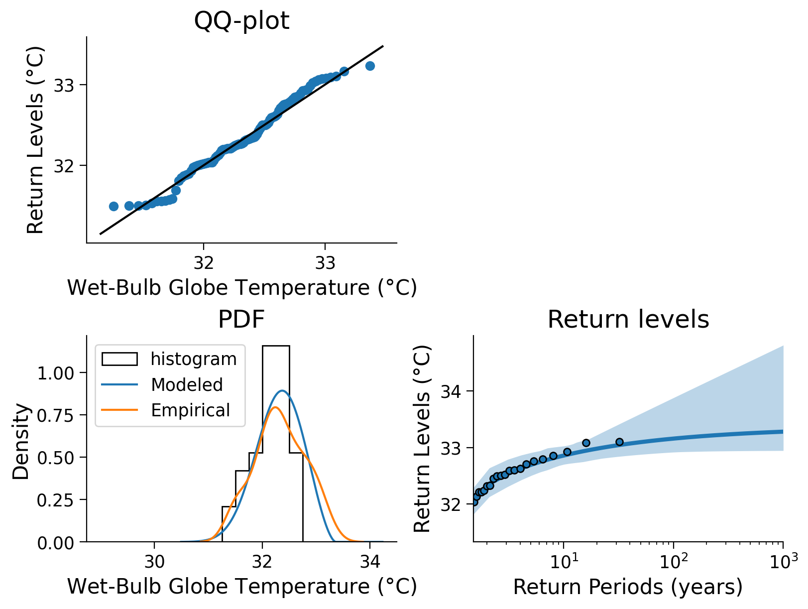
../../../_images/ad9a59624074657fe79a1909cc20e1b7d10118ecaf1d3107431fa2f4152dad14.png

Click here for a detailed description of the plot.

Top left: The QQ-plot shows the quantiles versus the return levels both in $\degree$C, calculated from the wet-bulb globe temperature data and emphasized as blue dots. For small quantiles, the return levels follow the identity line (black) less, additionally, in a few larger quantiles corresponding return levels increase with a smaller slope than the id line. This indicates a slight difference in the distributions of the two properties.

Bottom left: A comparison between modeled and empirical probability density functions (PDFs) shows slightly different distributions. The empirical PDF weights the density of larger anomalies more, so it appears that the GEV PDF underestimates large wet-bulb globe temperatures. In addition, the modeled scale parameter yields a higher maximum than the empirical estimate. The tails are comparable, however the empirical PDF sees more events in the extremes, especially in the maximum range.

Bottom right: The fitted return levels of the wet-bulb globe temperatures in $\degree$C versus return periods log-scaled in years. Blue dots highlight the empirical calculations (using the algorithm introduced in Tutorial 2), while the blue line emphasizes the fitted GEV corresponding relationship. Shaded areas represent the uncertainty ranges that were calculated with a bootstrap approach before. The larger the return periods, the less data on such events is given, hence the uncertainty increases.

# X-year of interest
x = 100
print(
    "{}-year return level: {:.2f} C".format(x,
        gf.estimate_return_level_period(x, loc_245, scale_245, shape_245).mean()
    )
)

100-year return level: 33.16 C

Compute as well the fit and return levels for the remaining two scenarios (SSP-126 and SSP-585). Save the QQ plot etc. for your own testing later on.

You can then plot all return level curves together to compare.

return_levels_126 = gf.fit_return_levels(
    wetbulb_126_delhi.sel(time=slice("2070", "2100")).values,
    years=np.arange(1.1, 1000),
    N_boot=100,
)
return_levels_585 = gf.fit_return_levels(
    wetbulb_585_delhi.sel(time=slice("2070", "2100")).values,
    years=np.arange(1.1, 1000),
    N_boot=100,
)

Location: 3.2e+01, scale: 5.0e-01, shape: 3.1e-01

Ranges with alpha=0.050 :
Location: [31.19 , 31.91]
Scale: [0.29 , 0.87]
Shape: [-0.52 , 1.15]
Location: 3.3e+01, scale: 1.1e+00, shape: 3.3e-01

Ranges with alpha=0.050 :
Location: [33.06 , 33.83]
Scale: [0.70 , 1.34]
Shape: [0.04 , 0.68]

fig, ax = plt.subplots()
gf.plot_return_levels(return_levels_hist, c="k", label="historical", ax=ax)
gf.plot_return_levels(return_levels_126, c="C0", label="ssp126", ax=ax)
gf.plot_return_levels(return_levels_245, c="C1", label="ssp245", ax=ax)
gf.plot_return_levels(return_levels_585, c="C2", label="ssp585", ax=ax)

ax.set_xlim(1, 100)
ax.set_ylim(29.5, 37)
ax.legend()
ax.grid(True, which="both")
ax.set_xlabel("Return Period (years)")
ax.set_ylabel("Return Level ($\degree$ C)")

Text(0, 0.5, 'Return Level ($\\degree$ C)')

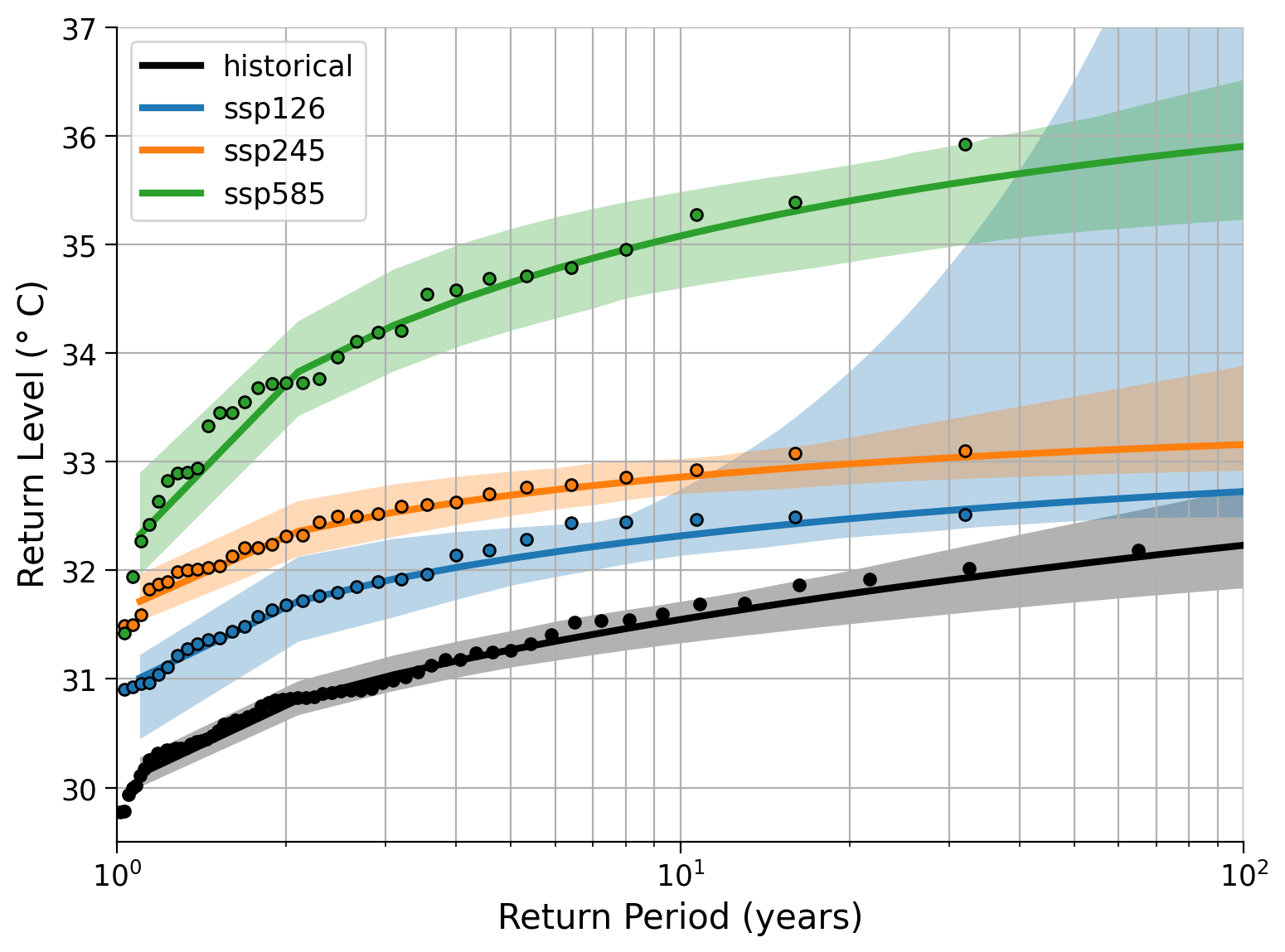
../../../_images/746b6acdbeeae82e12831087656a1d4767cd6a5419c4a4480c1bcbff7954b66c.png

Click here for a description of the plot.

The fitted return levels of the wet-bulb globe temperatures in $\degree$C versus return periods log-scaled in years for all four scenarios. Dots highlight the empirical calculations (using the algorithm introduced in Tutorial 2), while lines emphasize the fitted GEV corresponding relationship, respectively. Shaded areas represent the uncertainty ranges that were calculated with a bootstrap approach before. The larger the return periods, the less data on such events is given, hence the uncertainty increases.

Questions 1.1#

Compare the common event (return period << 10 years) to the very rare event (return period ~ 100 years) events under the different scenarios.

What is the return level of a 3-year event under the SSP5-8.5 scenario? Note down the level. What would be the return period of such an event in the other scenarios?
What is the return level of a 100-year event in the historical scenario. How often would such an event occur under the other scenarios?

Click for solution

Section 1.2: Return Levels Over Different Intervals#

Besides the late period (2070-2011), we compute the return levels over the near future (2015-2050). Then let’s plot the time series, and overlay the 100-year return level, as computed over 2015-2050, 2070-2100, and the historical period:

return_levels_126_2015_2050 = gf.fit_return_levels(
    wetbulb_126_delhi.sel(time=slice("2015", "2050")).values,
    years=np.arange(1.1, 1000),
    N_boot=100,
)
return_levels_245_2015_2050 = gf.fit_return_levels(
    wetbulb_245_delhi.sel(time=slice("2015", "2050")).values,
    years=np.arange(1.1, 1000),
    N_boot=100,
)
return_levels_585_2015_2050 = gf.fit_return_levels(
    wetbulb_585_delhi.sel(time=slice("2015", "2050")).values,
    years=np.arange(1.1, 1000),
    N_boot=100,
)

Location: 3.2e+01, scale: 4.9e-01, shape: 3.6e-01

Ranges with alpha=0.050 :
Location: [31.37 , 31.75]
Scale: [0.35 , 0.60]
Shape: [0.00 , 0.65]
Location: 3.1e+01, scale: 5.5e-01, shape: 2.4e-01

Ranges with alpha=0.050 :
Location: [31.02 , 31.52]
Scale: [0.44 , 0.70]
Shape: [0.00 , 0.45]
Location: 3.1e+01, scale: 4.4e-01, shape: 1.8e-01

Ranges with alpha=0.050 :
Location: [31.36 , 31.66]
Scale: [0.31 , 0.53]
Shape: [0.00 , 0.47]

fig, ax = plt.subplots()
# calculate annual mean for all scenarios and plot time series
wetbulb_hist_delhi.groupby("time.year").mean().plot.line(
    alpha=0.5, c="k", label="hist", ax=ax
)
wetbulb_126_delhi.groupby("time.year").mean().plot.line(
    alpha=0.5, c="C0", label="ssp126", ax=ax
)
wetbulb_245_delhi.groupby("time.year").mean().plot.line(
    alpha=0.5, c="C1", label="ssp245", ax=ax
)
wetbulb_585_delhi.groupby("time.year").mean().plot.line(
    alpha=0.5, c="C2", label="ssp585", ax=ax
)
# aesthetics
ax.set_title("")
ax.legend()

# add horizontal lines of 100 year event return levels for certain periods
# historical 1950-2014
ax.hlines(
    return_levels_hist.GEV.sel(period=100, method="nearest").values,
    1950,
    2014,
    "k",
    linestyle="-.",
    lw=2,
)
# SSP1-2.6 2015-2050
ax.hlines(
    return_levels_126_2015_2050.GEV.sel(period=100, method="nearest").values,
    2015,
    2050,
    "C0",
    linestyle="--",
    lw=2,
)
# SSP2-4.5 2015-2050
ax.hlines(
    return_levels_245_2015_2050.GEV.sel(period=100, method="nearest").values,
    2015,
    2050,
    "C1",
    linestyle="--",
    lw=2,
)
# SSP5-8.5 2015-2050
ax.hlines(
    return_levels_585_2015_2050.GEV.sel(period=100, method="nearest").values,
    2015,
    2050,
    "C2",
    linestyle="--",
    lw=2,
)
# SSP1-2.6 2070-2100
ax.hlines(
    return_levels_126.GEV.sel(period=100, method="nearest").values,
    2070,
    2100,
    "C0",
    linestyle=":",
    lw=2,
)
# SSP2-4.5 2070-2100
ax.hlines(
    return_levels_245.GEV.sel(period=100, method="nearest").values,
    2070,
    2100,
    "C1",
    linestyle=":",
    lw=2,
)
# SSP5-8.5 2070-2100
ax.hlines(
    return_levels_585.GEV.sel(period=100, method="nearest").values,
    2070,
    2100,
    "C2",
    linestyle=":",
    lw=2,
)
# aesthetics
plt.title("")
plt.xlabel("Time (years)")
plt.ylabel("Maximum 7-day Mean\nWet-Bulb Globe Temperature ($\degree$C)")

Text(0, 0.5, 'Maximum 7-day Mean\nWet-Bulb Globe Temperature ($\\degree$C)')

../../../_images/53df63a6c05c1dd93fcfc7e1909315525df09c892db1c2d2807f46b097faa3fb.png

Click here for a detailed description of the plot.

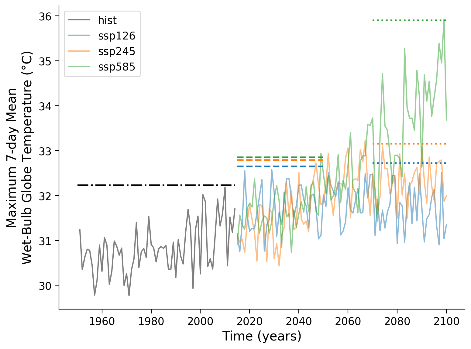
Time series of the wet-bulb globe temperature in $\degree$C in India, New Delhi for three scenarios and the historical period, overlaid by the 100-year return level of certain periods, as computed over 1950-2014 (dot-dashed), 2015-2050 (dashed), and 2070-2100 (dotted). In summary, the return levels increase over time, only the blue scenario (SSP1-2.6) keeps it at a temporally constant level at the end of the century, while the more severe scenarios still show rising return levels. The SSP5-8.5, often called the 'business-as-usual' scenario due to omitted implementation of policies, shows a return level of 36 $\degree$C for 100-year events, 3 years more than the SSP2-4.5 scenario.

Section 1.3: Time-Dependent Return Levels#

Looking at the previous plot we see trends present in our datasets, with the 100-year event return levels varying across the time periods we have choosen. This suggests that our location parameter is changing with time.

Now, similar to the previous tutorial, we assume that the location parameter is a function of time and proceed to estimate the GEV distribution for the four scenarios:

def estimate_return_level_model(quantile, model):
    loc, scale, shape = model.loc, model.scale, model.shape
    level = loc - scale / shape * (1 - (-np.log(quantile)) ** (-shape))
    return level

# fit the GEV to the data, while specifying that the location parameter ('loc') is meant
# to be a covariate ('c_') of the time axis (data.index)

law_ns_hist = sd.GEV()
for i in range(250):
    law_ns_hist.fit(wetbulb_hist_delhi.values, c_loc=np.arange(wetbulb_hist_delhi.time.size))
    #print(law_ns_hist.coef_)
    # if the first coefficient is not zero, we stop fitting
    if law_ns_hist.coef_[0] != 0:
        print(f'Found non-trivial solution for law_ns_hist after {i} fitting iterations.')
        print(law_ns_hist.coef_)
        break


law_ns_126 = sd.GEV()
for i in range(250):
    law_ns_126.fit(wetbulb_126_delhi.values, c_loc=np.arange(wetbulb_126_delhi.time.size))
    # if the first coefficient is not zero, we stop fitting
    if law_ns_126.coef_[0] != 0:
        print(f'Found non-trivial solution for law_ns_126 after {i} fitting iterations.')
        print(law_ns_126.coef_)
        break

law_ns_245 = sd.GEV()
for i in range(250):
    law_ns_245.fit(wetbulb_245_delhi.values, c_loc=np.arange(wetbulb_245_delhi.time.size))
    # if the first coefficient is not zero, we stop fitting
    if law_ns_245.coef_[0] != 0:
        print(f'Found non-trivial solution for law_ns_245 after {i} fitting iterations.')
        print(law_ns_245.coef_)
        break

law_ns_585 = sd.GEV()
for i in range(250):
    law_ns_585.fit(wetbulb_585_delhi.values, c_loc=np.arange(wetbulb_585_delhi.time.size))
    # if the first coefficient is not zero, we stop fitting
    if law_ns_585.coef_[0] != 0:
        print(f'Found non-trivial solution for law_ns_585 after {i} fitting iterations.')
        print(law_ns_585.coef_)
        break

fig, ax = plt.subplots()
wetbulb_hist_delhi.plot.line(c="k", ax=ax)
wetbulb_126_delhi.plot.line(c="C0", ax=ax)
wetbulb_245_delhi.plot.line(c="C1", ax=ax)
wetbulb_585_delhi.plot.line(c="C2", ax=ax)

ax.plot(
    wetbulb_hist_delhi.time,
    estimate_return_level_model(1 - 1 / 100, law_ns_hist),
    "k--",
    label="100-year return level: hist",
)
ax.plot(
    wetbulb_126_delhi.time,
    estimate_return_level_model(1 - 1 / 100, law_ns_126),
    "C0--",
    label="100-year return level: ssp126",
)
ax.plot(
    wetbulb_245_delhi.time,
    estimate_return_level_model(1 - 1 / 100, law_ns_245),
    "C1--",
    label="100-year return level: ssp245",
)
ax.plot(
    wetbulb_585_delhi.time,
    estimate_return_level_model(1 - 1 / 100, law_ns_585),
    "C2--",
    label="100-year return level: ssp585",
)

ax.legend()
ax.set_title("")
ax.set_xlabel("Time (years)")
ax.set_ylabel("Maximum 7-day Mean\nWet-Bulb Globe Temperature ($\degree$C)")

Now we again compute the AIC for the constant and time-dependent models, and compare their performance:

def compute_aic(model):
    return 2 * len(model.coef_) + 2 * model.info_.mle_optim_result.fun

# compute stationary models:
law_ss_hist = sd.GEV()
law_ss_hist.fit(wetbulb_hist_delhi.values)

law_ss_126 = sd.GEV()
law_ss_126.fit(wetbulb_126_delhi.values)

law_ss_126 = sd.GEV()
law_ss_126.fit(wetbulb_126_delhi.values)

law_ss_245 = sd.GEV()
law_ss_245.fit(wetbulb_245_delhi.values)

law_ss_585 = sd.GEV()
law_ss_585.fit(wetbulb_585_delhi.values)

aics = pd.DataFrame(
    columns=["hist", "ssp126", "ssp245", "ssp585"], index=["constant", "covariate"]
)

aics["hist"] = compute_aic(law_ss_hist), compute_aic(law_ns_hist)
aics["ssp126"] = compute_aic(law_ss_126), compute_aic(law_ns_126)
aics["ssp245"] = compute_aic(law_ss_245), compute_aic(law_ns_245)
aics["ssp585"] = compute_aic(law_ss_585), compute_aic(law_ns_585)

aics.round(2)

	hist	ssp126	ssp245	ssp585
constant	NaN	NaN	NaN	NaN
covariate	NaN	NaN	NaN	NaN

The AIC is lower when using a covariate, suggesting that including the time dependence in the location parameter improves the quality of the model. The exception is the SSP1-2.6 scenario, which does not perform as well. This is because, unlike the other scenarios and the historical period, the wet-bulb globe temperatures stabilize, hence this location parameter is less dependent on time. In this instance, making other parameters depend on time could potentially improve the performance.

Section 2: Spatial Analysis#

After looking at New Delhi, India, now we can make use of the spatial information:

The code provided below is commented and is used to fit the GEV distribution for each grid point. For the historical scenario, the entire time range is used, while for the selected scenarios, the period from 2071 to 2100 (the last 30 years of the data) is used.

Please note that the computation for this code takes some time (approximately 9 minutes per dataset). To save time, we have already precomputed the data, so there is no need to run the commented code. However, you are free to uncomment and run the code, make modifications, or include time-dependent parameters (as shown above) at your convenience. If desired, you can also focus on specific regions.

Expensive code that fits a GEV distribution to each grid point:

# this code requires the authors' extremes_functions.py file and SDFC library from github: https://github.com/yrobink/SDFC
# The code takes roughly 30 minutes to execute, in the next cell we load in the precomputed data. Uncomment the following lines if you want to rerun.
# fit_sp_hist = ef.fit_return_levels_sdfc_2d(wetbulb_hist.rename({'lon':'longitude','lat':'latitude'}),times=np.arange(1.1,1000),periods_per_year=1,kind='GEV',N_boot=0,full=True)
# fit_sp_126 = ef.fit_return_levels_sdfc_2d(wetbulb_126.sel(time=slice('2071','2100')).rename({'lon':'longitude','lat':'latitude'}),times=np.arange(1.1,1000),periods_per_year=1,kind='GEV',N_boot=0,full=True)
# fit_sp_245 = ef.fit_return_levels_sdfc_2d(wetbulb_245.sel(time=slice('2071','2100')).rename({'lon':'longitude','lat':'latitude'}),times=np.arange(1.1,1000),periods_per_year=1,kind='GEV',N_boot=0,full=True)
# fit_sp_585 = ef.fit_return_levels_sdfc_2d(wetbulb_585.sel(time=slice('2071','2100')).rename({'lon':'longitude','lat':'latitude'}),times=np.arange(1.1,1000),periods_per_year=1,kind='GEV',N_boot=0,full=True)

Section 2.1: Load Pre-Computed Data#

# historical - wbgt_hist_raw_runmean7_gev.nc
fname_wbgt_hist = "wbgt_hist_raw_runmean7_gev.nc"
url_wbgt_hist = "https://osf.io/dakv3/download"
fit_sp_hist = xr.open_dataset(pooch_load(url_wbgt_hist, fname_wbgt_hist))

# SSP-126 - wbgt_126_raw_runmean7_gev_2071-2100.nc
fname_wbgt_126 = "wbgt_126_raw_runmean7_gev_2071-2100.nc"
url_wbgt_126 = "https://osf.io/ef9pv/download"
fit_sp_126 = xr.open_dataset(pooch_load(url_wbgt_126, fname_wbgt_126))

# SSP-245 - wbgt_245_raw_runmean7_gev_2071-2100.nc
fname_wbgt_245 = "wbgt_245_raw_runmean7_gev_2071-2100.nc"
url_wbgt_245 = "https://osf.io/j4hfc/download"
fit_sp_245 = xr.open_dataset(pooch_load(url_wbgt_245, fname_wbgt_245))

# SSP-585 - wbgt_585_raw_runmean7_gev_2071-2100.nc
fname_bgt_58 = "wbgt_585_raw_runmean7_gev_2071-2100.nc"
url_bgt_585 = "https://osf.io/y6edw/download"
fit_sp_585 = xr.open_dataset(pooch_load(url_bgt_585, fname_bgt_58))

Downloading data from 'https://osf.io/dakv3/download' to file '/tmp/wbgt_hist_raw_runmean7_gev.nc'.

SHA256 hash of downloaded file: d81109ded24b8a2f8846364bbcdeca22a187d0b5c5cbe908599f9fa32b1f1152
Use this value as the 'known_hash' argument of 'pooch.retrieve' to ensure that the file hasn't changed if it is downloaded again in the future.

Downloading data from 'https://osf.io/ef9pv/download' to file '/tmp/wbgt_126_raw_runmean7_gev_2071-2100.nc'.

SHA256 hash of downloaded file: b98318842c15c16ee03fb23faca965abf18f78b862857f6109d6a6e073b86301
Use this value as the 'known_hash' argument of 'pooch.retrieve' to ensure that the file hasn't changed if it is downloaded again in the future.

Downloading data from 'https://osf.io/j4hfc/download' to file '/tmp/wbgt_245_raw_runmean7_gev_2071-2100.nc'.

SHA256 hash of downloaded file: 1e5cd5ef92336b23ad0c8d51c3cebfc87374d57ce375969d79243aff43c67b2f
Use this value as the 'known_hash' argument of 'pooch.retrieve' to ensure that the file hasn't changed if it is downloaded again in the future.

Downloading data from 'https://osf.io/y6edw/download' to file '/tmp/wbgt_585_raw_runmean7_gev_2071-2100.nc'.

SHA256 hash of downloaded file: 916063b8695dbf2e0c2cb630eeb6b36cb9c2b3cfe4912a45f2bc48837c11401c
Use this value as the 'known_hash' argument of 'pooch.retrieve' to ensure that the file hasn't changed if it is downloaded again in the future.

Also load the area for each grid box - we will use this later to compute global averages:

# filename - area_mpi.nc
filename_area_mpi = "area_mpi.nc"
url_area_mpi = "https://osf.io/zqd86/download"
area = xr.open_dataarray(pooch_load(url_area_mpi, filename_area_mpi))

# filename - area_land_mpi.nc
filename_area_mpi = "area_land_mpi.nc"
url_area_land_mpi = "https://osf.io/dxq98/download"
area_land = xr.open_dataarray(pooch_load(url_area_land_mpi, filename_area_mpi)).fillna(
    0.0
)

Downloading data from 'https://osf.io/zqd86/download' to file '/tmp/area_mpi.nc'.

SHA256 hash of downloaded file: 8c7235af276325bf7683af3da90c106ac48324241a6ad137a83fcea8eaa2938d
Use this value as the 'known_hash' argument of 'pooch.retrieve' to ensure that the file hasn't changed if it is downloaded again in the future.

Downloading data from 'https://osf.io/dxq98/download' to file '/tmp/area_land_mpi.nc'.

SHA256 hash of downloaded file: 640613a7d608681804df67d6d480f09690da32de189184a774ff74773240c2aa
Use this value as the 'known_hash' argument of 'pooch.retrieve' to ensure that the file hasn't changed if it is downloaded again in the future.

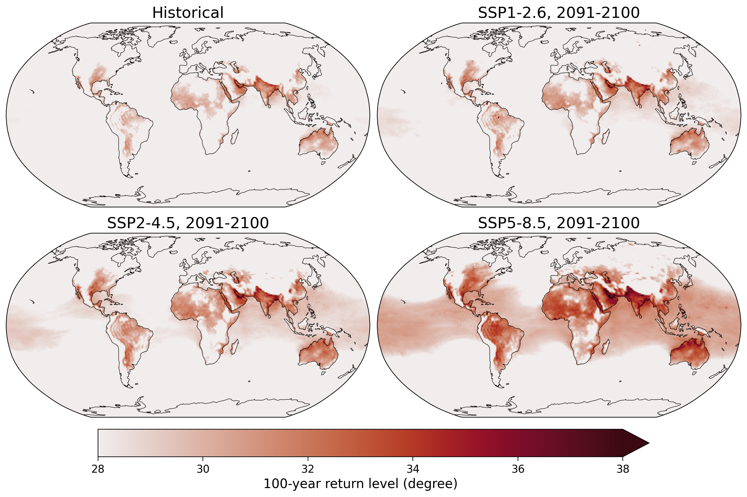
Now, let’s examine the 100-year return level in the historical run and compare it to the period from 2071-2100 in the three scenarios. The colorbar has been set to start at 28 $\degree$C, which is approximately the temperature reached during the severe heatwaves in Europe in 2003 and Russia in 2010.

# setup plots
fig, axs = plt.subplots(
    2,
    2,
    constrained_layout=True,
    figsize=(12, 8),
    subplot_kw=dict(projection=ccrs.Robinson()),
)
# reduce axis dimension to have one index only
ax = axs.flatten()

# summarize all kwargs used for al plots
kwargs = dict(
    vmin=28, vmax=38, cmap=cmo.amp, transform=ccrs.PlateCarree(), add_colorbar=False
)

# select 100-year event for every grid cell in every scenario dataset
p = (
    fit_sp_hist["return level"]
    .sel({"return period": 100}, method="nearest")
    .plot(ax=ax[0], **kwargs)
)
fit_sp_126["return level"].sel({"return period": 100}, method="nearest").plot(
    ax=ax[1], **kwargs
)
fit_sp_245["return level"].sel({"return period": 100}, method="nearest").plot(
    ax=ax[2], **kwargs
)
fit_sp_585["return level"].sel({"return period": 100}, method="nearest").plot(
    ax=ax[3], **kwargs
)

# define colorbar
cbar = fig.colorbar(
    p,
    ax=ax,
    pad=0.025,
    orientation="horizontal",
    shrink=0.75,
    label="100-year return level (degree)",
    extend="max",
)

# aesthetics for all subplots
ax[0].set_title("Historical")
ax[1].set_title("SSP1-2.6, 2091-2100")
ax[2].set_title("SSP2-4.5, 2091-2100")
ax[3].set_title("SSP5-8.5, 2091-2100")

[axi.set_facecolor("grey") for axi in ax]
[axi.coastlines(lw=0.5) for axi in ax]

[<cartopy.mpl.feature_artist.FeatureArtist at 0x7fe21bbff5e0>,
 <cartopy.mpl.feature_artist.FeatureArtist at 0x7fe21bb9dca0>,
 <cartopy.mpl.feature_artist.FeatureArtist at 0x7fe21bbe2460>,
 <cartopy.mpl.feature_artist.FeatureArtist at 0x7fe21bbe2a30>]

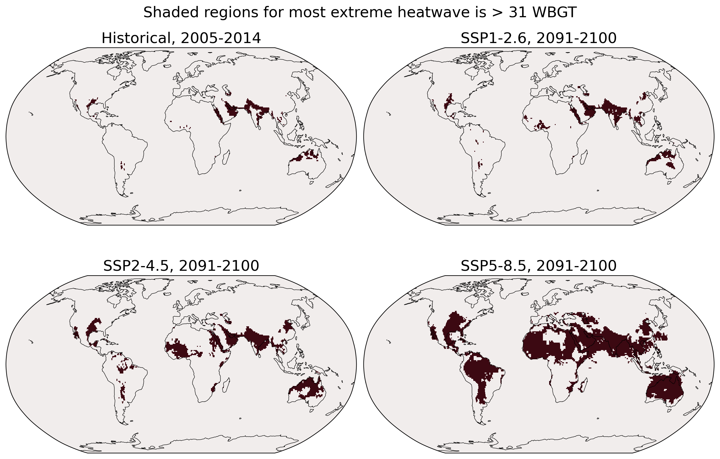
../../../_images/42e376b3482a6b4bf24aff4bef41f70e8705c62947eaf89b9ee7b9a04d032155.png

In the following regions where the hottest heatwave is above 31 degrees wet-bulb globe temperature are given by the red shading, which is considered a “critical temperature” above which a human will die within a few hours without non-evaporative cooling like air conditioning:

fig, axs = plt.subplots(
    2,
    2,
    constrained_layout=True,
    figsize=(12, 8),
    subplot_kw=dict(projection=ccrs.Robinson()),
)
ax = axs.flatten()

kwargs = dict(vmin=0, cmap=cmo.amp, transform=ccrs.PlateCarree(), add_colorbar=False)

p = (wetbulb_hist.sel(time=slice("2005", "2014")).max("time") > 31).plot(
    ax=ax[0], **kwargs
)
(wetbulb_126.sel(time=slice("2091", "2100")).max("time") > 31).plot(ax=ax[1], **kwargs)
(wetbulb_245.sel(time=slice("2091", "2100")).max("time") > 31).plot(ax=ax[2], **kwargs)
(wetbulb_585.sel(time=slice("2091", "2100")).max("time") > 31).plot(ax=ax[3], **kwargs)

# cbar = fig.colorbar(p,ax=ax,pad=0.025,orientation='horizontal',shrink=0.75,label='Most extreme 7-day mean WBGT')

ax[0].set_title("Historical, 2005-2014")
ax[1].set_title("SSP1-2.6, 2091-2100")
ax[2].set_title("SSP2-4.5, 2091-2100")
ax[3].set_title("SSP5-8.5, 2091-2100")

[axi.set_facecolor("grey") for axi in ax]
[axi.coastlines(lw=0.5) for axi in ax]

fig.suptitle("Shaded regions for most extreme heatwave is > 31 WBGT")

Text(0.5, 0.98, 'Shaded regions for most extreme heatwave is > 31 WBGT')

../../../_images/432f71fb324dfb95ec85a326bd2d7c8422e0cd8147d8e399a01cb5d84aa5a879.png

Now we will examine the changes over time in the portion of the Earth’s land surface affected by extreme heatwaves. To accomplish this, we utilize the previously loaded grid box area data.

Next, we assign a value of “1” to the temporal-spatial data if it surpasses the defined threshold, and a value of “0” if it does not. By conducting an area-weighted average across the entire land area of the world, we determine the fraction of land area experiencing a heatwave above the threshold for each year.

fig, ax = plt.subplots()
((wetbulb_hist > 31) * 1).weighted(area_land).mean(["lon", "lat"]).plot.line(
    "k.-", label="historical", ax=ax
)
((wetbulb_126 > 31) * 1).weighted(area_land).mean(["lon", "lat"]).plot.line(
    ".-", label="ssp126", ax=ax
)
((wetbulb_245 > 31) * 1).weighted(area_land).mean(["lon", "lat"]).plot.line(
    ".-", label="ssp245", ax=ax
)
((wetbulb_585 > 31) * 1).weighted(area_land).mean(["lon", "lat"]).plot.line(
    ".-", label="ssp585", ax=ax
)

ax.grid(True)

ax.legend()
ax.set_xlabel("Time (years)")
ax.set_ylabel("Land Area Fraction")
ax.set_title("Fraction of land area\nwith 7 days of wet-bulb temperature > 31 degrees")

Text(0.5, 1.0, 'Fraction of land area\nwith 7 days of wet-bulb temperature > 31 degrees')

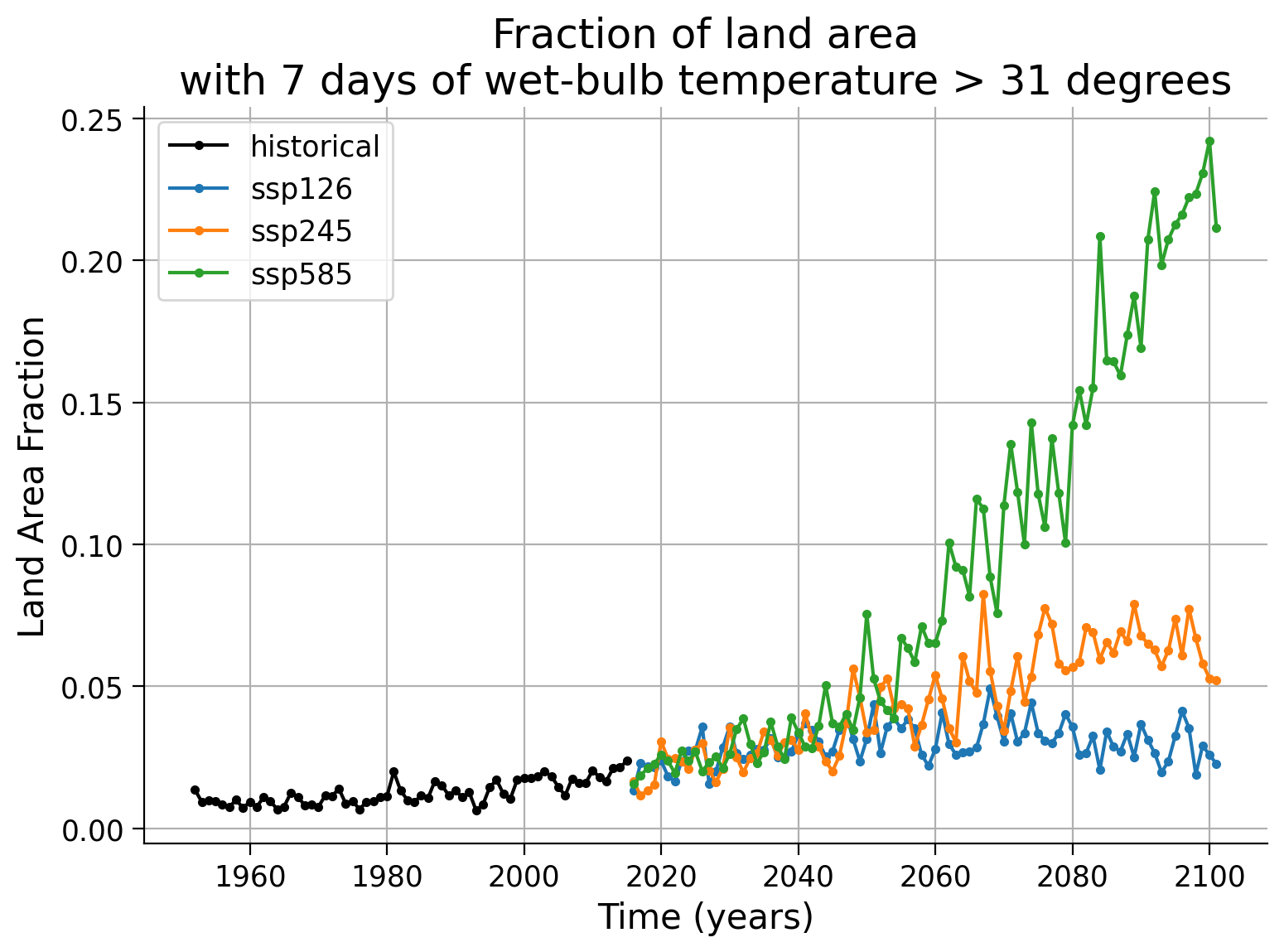
../../../_images/1f71a18923347f65bc217b211ebd231d41a17333c4e11463f01591160c5fe5d1.png

Let’s average the fraction of the land area of the world that experiences a heatwave above wet-bulb temperature of 31 in the last 10 years of each run.

print(
    "Fraction of the land area of the world that experiences a heatwave above wet-bulb temperature of 31 in the last 10 years of each run in percent:"
)
(
    pd.Series(
        index=["historical", "SSP-126", "SSP-245", "SSP-585"],
        data=[
            ((wetbulb_hist > 31) * 1)
            .weighted(area_land)
            .mean(["lon", "lat"])
            .isel(time=slice(-10, None))
            .mean()
            .values,
            ((wetbulb_126 > 31) * 1)
            .weighted(area_land)
            .mean(["lon", "lat"])
            .isel(time=slice(-10, None))
            .mean()
            .values,
            ((wetbulb_245 > 31) * 1)
            .weighted(area_land)
            .mean(["lon", "lat"])
            .isel(time=slice(-10, None))
            .mean()
            .values,
            ((wetbulb_585 > 31) * 1)
            .weighted(area_land)
            .mean(["lon", "lat"])
            .isel(time=slice(-10, None))
            .mean()
            .values,
        ],
    ).astype(float)
    * 100
).round(2)

Fraction of the land area of the world that experiences a heatwave above wet-bulb temperature of 31 in the last 10 years of each run in percent:

historical     1.82
SSP-126        2.75
SSP-245        6.24
SSP-585       21.89
dtype: float64

Questions 2.1#

What observations can you make when examining the time evolution and comparing the different scenarios?
Do you think these results would change if you used a different threshold such as 28 or 33 degrees? Why would it be important to look at this?

Click for solution

Summary#

In this tutorial, you learned what the wet-bulb globe temperature is and how it affects human health. You analyzed the likelihood of crossing critical thresholds under historical and future climate scenarios, using data from a specific climate model. You learned how to conduct a spatial GEV analysis and evaluated the potential human impact under extreme heat waves.

Resources#

The data for this tutorial was accessed through the Pangeo Cloud platform.

This tutorial uses data from the simulations conducted as part of the CMIP6 multi-model ensemble, in particular the models MPI-ESM1-2-HR.

MPI-ESM1-2-HR was developed and the runs were conducted by the Max Planck Institute for Meteorology in Hamburg, Germany.

For references on particular model experiments see this database.

For more information on what CMIP is and how to access the data, please see this page.

Bonus Tutorial 8: Thresholds

Contents

Bonus Tutorial 8: Thresholds#

Tutorial Objectives#

Setup#

Figure Settings#

Helper functions#

Video 1: Thresholds#

Section 1: Downloading the Data#

Section 1.1: Focus on New Delhi, India#

Questions 1.1#

Section 1.2: Return Levels Over Different Intervals#

Section 1.3: Time-Dependent Return Levels#

Section 2: Spatial Analysis#

Section 2.1: Load Pre-Computed Data#

Questions 2.1#

Summary#

Resources#