Tutorial 2: Future climate scenarios & Multi-model Ensembles

Tutorial 2: Future climate scenarios & Multi-model Ensembles#

Week 2, Day 1, An Ensemble of Futures

Content creators: Brodie Pearson, Julius Busecke, Tom Nicholas, Sam Ditkovsky

Content reviewers: Mujeeb Abdulfatai, Nkongho Ayuketang Arreyndip, Jeffrey N. A. Aryee, Younkap Nina Duplex, Sloane Garelick, Paul Heubel, Zahra Khodakaramimaghsoud, Peter Ohue, Jenna Pearson, Abel Shibu, Derick Temfack, Peizhen Yang, Cheng Zhang, Chi Zhang, Ohad Zivan

Content editors: Paul Heubel, Jenna Pearson, Ohad Zivan, Chi Zhang

Production editors: Wesley Banfield, Paul Heubel, Jenna Pearson, Konstantine Tsafatinos, Chi Zhang, Ohad Zivan

Our 2024 Sponsors: CMIP, NFDI4Earth

Tutorial Objectives#

Estimated timing for tutorial: 40 minutes

In this tutorial, we will analyze data from five different CMIP6 models developed by various institutions around the world, focusing on their historical simulations and low-emission projections (SSP1-2.6). By the end of this tutorial, you will be able to

Load CMIP6 Sea Surface Temperature (SST) data from multiple models;
Calculate the SST anomalies, and recall the concept of temperature anomaly in relation to a base period

Setup#

# installations ( uncomment and run this cell ONLY when using google colab or kaggle )

# !pip install condacolab &> /dev/null
# import condacolab
# condacolab.install()

# # Install all packages in one call (+ use mamba instead of conda), this must in one line or code will fail
# !mamba install xarray-datatree intake-esm gcsfs xmip aiohttp nc-time-axis cf_xarray xarrayutils &> /dev/null

# imports
import intake
import matplotlib.pyplot as plt
import xarray as xr

from xmip.preprocessing import combined_preprocessing
from xmip.postprocessing import _parse_metric
from datatree import DataTree

/opt/hostedtoolcache/Python/3.9.19/x64/lib/python3.9/site-packages/esmpy/interface/loadESMF.py:94: VersionWarning: ESMF installation version 8.7.0 beta snapshot, ESMPy version 8.7.0b9
  warnings.warn("ESMF installation version {}, ESMPy version {}".format(

Install and import feedback gadget#

Figure settings#

Helper functions#

Video 1: Why So Many Earth System Models?#

Submit your feedback#

If you want to download the slides: https://osf.io/download/3sa5z/

Submit your feedback#

Section 1: Load CMIP6 SST Data from Five Models and Three Experiments#

In the previous section, you investigated the internal variability in a single CMIP6 model (TaiESM1) simulated past temperature.

Now we will start to analyze a multi-model ensemble that consists of data from multiple CMIP6 models, and includes both historical simulations and future scenario projections.

Your multi-model ensemble will consist of Five different CMIP6 models developed by institutions from a variety of countries:

TaiESM1 (Research Center for Environmental Changes, Taiwan),
IPSL-CM6A-LR (Institut Pierre Simon Laplace, France),
GFDL-ESM4 (NOAA Geophysical Fluid Dynamics Laboratory, USA),
ACCESS-CM2 (CSIRO and ARCCSS, Australia), and
MPI-ESM1-2-LR (Max Planck Institute, Germany).

We can specify these models through the source_id facet. You can see a table of CMIP6 source_id values here, and you can learn more about CMIP through our CMIP Resource Bank and the CMIP website.

Note that these are only a subset of the dozens of models, institutes, countries, and experiments that contribute to CMIP6, as discussed in the previous W2D1 Tutorial 2 video. Some of the abbreviations in the model names refer to institutes (MPI/GFDL), while some refer to the complexity and version of the model (e.g., Earth System or Climate Model [ESM/CM] and low- or high-resolution [LR/HR]). There are often several models from a single institute with each having a distinct level of complexity.

# selected CMIP6 models to explore
source_ids = ["IPSL-CM6A-LR", "GFDL-ESM4", "ACCESS-CM2", "MPI-ESM1-2-LR", "TaiESM1"]

# dictionary of facets for query of surface temperature data
facet_dict = { "source_id":source_ids,
    "variable_id":"tos",
    "member_id":"r1i1p1f1",
    "table_id":"Omon",
    "grid_label":"gn",
    "experiment_id":["historical", "ssp126", "ssp585"],
    "require_all_on":"source_id"
    }

# dictionary for query of cell area metric
facet_dict_area = { "source_id":source_ids,
    "variable_id":"areacello",
    "member_id":"r1i1p1f1",
    "table_id":"Ofx",
    "grid_label":"gn",
    "experiment_id":"historical",
    "require_all_on":"source_id"
    }

# search for temperature and area data and return datatree objects
dt = readin_cmip6_to_datatree(facet_dict)
dt_area = readin_cmip6_to_datatree(facet_dict_area)

# merge area metric into datatree object
dt_with_area = DataTree()
for model, subtree in dt.items():
    metric = dt_area[model]["historical"].ds["areacello"]
    dt_with_area[model] = subtree.map_over_subtree(_parse_metric, metric)

--> The keys in the returned dictionary of datasets are constructed as follows:
	'source_id/experiment_id'

100.00% [15/15 00:06<00:00]

--> The keys in the returned dictionary of datasets are constructed as follows:
	'source_id/experiment_id'

100.00% [5/5 00:01<00:00]

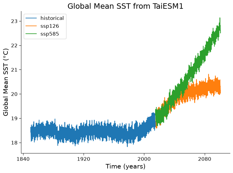
Let’s first reproduce the previous tutorial’s time series of Global Mean SST \(\left(GMSST\right)\) from TaiESM1 through the historical experiment and two future emissions scenarios

# average every dataset in the tree globally
dt_gm = dt_with_area.map_over_subtree(global_mean)

# create plot
fig, ax = plt.subplots()
# draw every scenario
for experiment in ["historical", "ssp126", "ssp585"]:
    da = dt_gm["TaiESM1"][experiment].ds.tos
    da.plot(label=experiment, ax=ax)

# aesthetics
ax.set_title("Global Mean SST from TaiESM1")
ax.set_ylabel("Global Mean SST (°C)")
ax.set_xlabel("Time (years)")
ax.legend()

<matplotlib.legend.Legend at 0x7f6d90b47790>

../../../_images/1101a2ce6a49a756e88bb451e6c20cc2938d0870ae0a31c3ffa8bd70790add9f.png

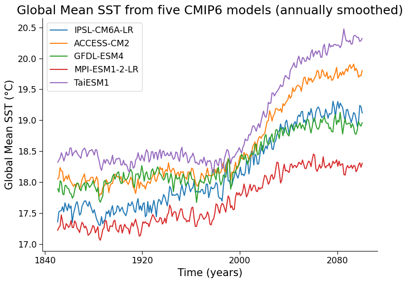
Coding Exercise 1.1: Combine past and future data, remove seasonal oscillations, and plot all 5 of the CMIP6 models we just loaded#

The historical and projected data are separate time series. Complete the xr.concat() function to combine the historical and projected data into a single continuous time series for each model.
The previous time series oscillated very rapidly due to Earth’s seasonal cycles. Finish the xarray .resample() function so that it smooths the monthly data with a one-year running mean. This will make it easier to distinguish the long-term changes in sea surface temperature.
Hint: this code is already set up to use all 5 of the CMIP6 models you just loaded, as it loops through and plots each model in the DataTree [dt.keys()]

#################################################
## TODO for students: Plot annually smoothed global mean SST for all models##
# please remove the following line of code once you have completed the exercise:
raise NotImplementedError("Student exercise: Plot annually smoothed global mean SST for all models")
#################################################


def plot_historical_ssp126_combined(dt, ax):
    for model in dt.keys():
        datasets = []
        for experiment in ["historical", "ssp126"]:
            datasets.append(dt[model][experiment].tos)

        # for each of the models, concatenate its historical and future data
        da_combined = xr.concat(...)
        # plot annual averages
        da_combined.coarsen(...).mean().plot(label=model, ax=ax)


fig, ax = plt.subplots()
# plot_historical_ssp126_combined
_ = ...

ax.set_title("Global Mean SST from five CMIP6 models (annually smoothed)")
ax.set_ylabel("Global Mean SST (°C)")
ax.set_xlabel("Time (years)")
ax.legend()

Click for solution

Example output:

Submit your feedback#

Question 1.1#

Why do you think the global mean temperature varies so much between models?*

*If you get stuck here, reflect on the videos from earlier today and the tutorials/videos from the Introduction to Climate Modeling day for inspiration.

Click for solution

Submit your feedback#

Coding Exercise 1.2#

As you just saw, the global mean SST varies between climate models. This is not surprising given the slight differences in physics, numerics, and discretization between each model.

When we are looking at future projections, we care about how each model has changed relative to their equilibrium/previous state. To do this, we typically subtract a historical reference period from the time series. This creates a new time series which we call the temperature anomaly relative to that period. Recall that you already calculated and used anomalies earlier in the course (e.g., on W1D1, Tutorial 6).

Modify the following code to recreate the previous multi-model figure, but now instead plot the global mean sea surface temperature (GMSST) anomaly relative to the 1950-1980 base period (i.e., subtract the 1950-1980 mean GMSST of each model from that model’s time series)

Hint: you will need to use ds.sel to select data during the base period (see here under “Indexing with dimension names” for a helpful example) along with the averaging operator, .mean().

#################################################
## TODO for students: Plot global mean SST anomaly for all models.##
# Please remove the following line of code once you have completed the exercise:
raise NotImplementedError("Student exercise: Plot global mean SST anomaly for all models.")
#################################################

# calculate anomaly to reference period
def datatree_anomaly(dt):
    dt_out = DataTree()
    for model, subtree in dt.items():
        # find the temporal average over the desired reference period
        ref = ...
        dt_out[model] = subtree - ref
    return dt_out

# apply anomaly function
dt_gm_anomaly = datatree_anomaly(dt_gm)

# create plot
fig, ax = plt.subplots()

# draw data with helper function
plot_historical_ssp126_combined(dt_gm_anomaly, ax)

# aesthetics
ax.set_title(
    "Global Mean SST Anomaly from five CMIP6 models (base period: 1950 to 1980)"
)
ax.set_ylabel("Global Mean SST Anomaly (°C)")
ax.set_xlabel("Time (years)")
ax.legend()

Click for solution

Example output:

Submit your feedback#

Questions 1.2: Climate Connection#

How does this figure compare to the previous one where the reference period was not subtracted?
This figure uses the reference period of 1950-1980 for its anomaly calculation. How does the variability across models 100 years before the base period (1850) compare to the variability 100 years after the base period (2080)? Why do you think this is?

Click for solution

Submit your feedback#

Summary#

In this tutorial, we expanded on the previous examination of a single CMIP6 model (TaiESM1 or MPI-ESM1-2-LR), to instead work with multi-model ensembles comprising five different CMIP6 models developed by institutions around the world (TaiESM1, IPSL-CM6A-LR, GFDL-ESM4, ACCESS-CM2, and MPI-ESM1-2-LR). We demonstrated the importance of anomalizing each of these models relative to a base period when calculating changes in the simulated Earth system. If variables are not anomalized, these absolute values can differ significantly between models due to the diversity of models (i.e., their distinct physics, numerics, and discretization).

Resources#

This tutorial uses data from the simulations conducted as part of the CMIP6 multi-model ensemble.

For examples on how to access and analyze data, please visit the Pangeo Cloud CMIP6 Gallery

For more information on what CMIP is and how to access the data, please see this page.

Tutorial 2: Future climate scenarios & Multi-model Ensembles

Contents

Tutorial 2: Future climate scenarios & Multi-model Ensembles#

Tutorial Objectives#

Setup#

Install and import feedback gadget#

Figure settings#

Helper functions#

Video 1: Why So Many Earth System Models?#

Submit your feedback#

Submit your feedback#

Section 1: Load CMIP6 SST Data from Five Models and Three Experiments#

Coding Exercise 1.1: Combine past and future data, remove seasonal oscillations, and plot all 5 of the CMIP6 models we just loaded#

Submit your feedback#

Question 1.1#

Submit your feedback#

Coding Exercise 1.2#

Submit your feedback#

Questions 1.2: Climate Connection#

Submit your feedback#

Summary#

Resources#