![]()

Bonus Tutorial 4: Climate Feedbacks#
Week 1, Day 5, Introduction to Climate Modeling
Content creators: Abigail Bodner, Jenna Pearson, Brodie Pearson, and Brian E. J. Rose
Content reviewers: Mujeeb Abdulfatai, Nkongho Ayuketang Arreyndip, Jeffrey N. A. Aryee, Younkap Nina Duplex, Will Gregory, Paul Heubel, Zahra Khodakaramimaghsoud, Peter Ohue, Agustina Pesce, Abel Shibu, Derick Temfack, Yunlong Xu, Peizhen Yang, Chi Zhang, Ohad Zivan
Content editors: Abigail Bodner, Paul Heubel, Brodie Pearson, Ohad Zivan, Chi Zhang
Production editors: Wesley Banfield, Paul Heubel, Jenna Pearson, Konstantine Tsafatinos, Chi Zhang, Ohad Zivan
Our 2024 Sponsors: CMIP, NFDI4Earth
Tutorial Objectives#
Estimated timing of tutorial: 30 minutes
Note that this and the two following tutorials contain solely Bonus content, that serves experienced participants and for later investigation of 0- and 1-dimensional models after the course. Please check out these tutorials after finishing Tutorial 7-8 successfully.
In this tutorial, students will learn about climate feedbacks, in particular the Planck and ice-albedo feedbacks. Students will also learn about how variations in the insolation over time can affect the equilibrium temperature of Earth.
By the end of this tutorial students will be able to:
Apply a temperature-dependent albedo within their existing climate model.
Understand the impact of insolation changes on the equilibrium temperature of Earth.
This tutorial draws on content from The Climate Laboratory by Brian E. J. Rose.
Setup#
# imports

import numpy as np                 # used for algebra and array operations
import matplotlib.pyplot as plt    # used for plotting
from scipy.optimize import brentq  # used for numerical root-finding to get the equilibria
Install and import feedback gadget#
Show code cell source
# @title Install and import feedback gadget

!pip3 install vibecheck datatops --quiet

from vibecheck import DatatopsContentReviewContainer
def content_review(notebook_section: str):
    return DatatopsContentReviewContainer(
        "",  # No text prompt
        notebook_section,
        {
            "url": "https://pmyvdlilci.execute-api.us-east-1.amazonaws.com/klab",
            "name": "comptools_4clim",
            "user_key": "l5jpxuee",
        },
    ).render()


feedback_prefix = "W1D5_T4"
Figure ettings#
Show code cell source
# @title Figure ettings
import ipywidgets as widgets  # interactive display

%config InlineBackend.figure_format = 'retina'
plt.style.use(
    "https://raw.githubusercontent.com/neuromatch/climate-course-content/main/cma.mplstyle"
)
Video 1: Climate Feedbacks#
Submit your feedback#
Show code cell source
# @title Submit your feedback
content_review(f"{feedback_prefix}_Climate_Feedbacks_Video")
If you want to download the slides: https://osf.io/download/btpwx/
Submit your feedback#
Show code cell source
# @title Submit your feedback
content_review(f"{feedback_prefix}_Climate_Feedbacks_Slides")
Section 1: Ice-Albedo Feedback#
Section 1.1: Temperature Dependent Albedo#
Our current model only contains one feedback, the ‘Planck feedback’ also called the ‘Planck temperature response’. This feedback encapsulates that a warming of Earth leads to the planet emitting more energy (see Planck’s law from Tutorial 1). In reality, there are many climate feedbacks that contribute to the Earth’s net temperature change due to an energy imbalance. In this tutorial, we will focus on incorporating an ice-albedo feedback into our model.
When the Earth’s surface warms, snow and ice melt. This lowers the albedo (\(\mathbf{\alpha}\)), because less solar radiation is reflected off Earth’s surface. This lower albedo causes the climate to warm even more than if the albedo had stayed the same, increasing the snow and ice melt. This is referred to as a positive feedback. Positive feedbacks amplify the changes that are already occurring. This particular feedback is referred to as the ice-albedo feedback.
A simple way to parameterize ice-albedo feedback in our model is through a temperature-dependent albedo, such as the one defined below (see the tutorial lecture slides for an explanation of why we use this function).
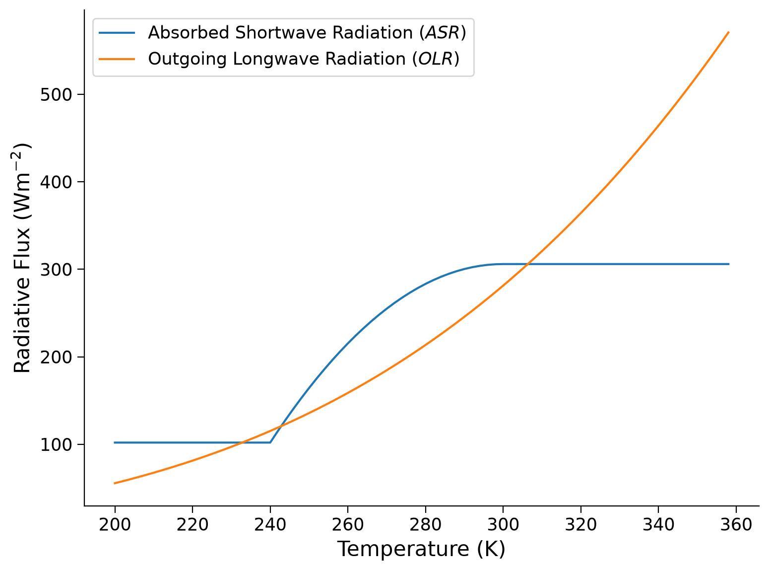
Using this new temperature-dependent albedo, we can plot the graphs of absorbed shortwave radiation \(\left(ASR\right)\) and outgoing longwave radiation \(\left(OLR\right)\):
# create a array ot temperatures to evaluates the ASR and OLR at
T = np.arange(200, 360, 2, dtype=np.float64)

# create empty arrays to fill with values later
ASR_vals = np.zeros_like(T)

# define the slope of the ramp function
m = (0.7 - 0.3) / (280 - 250)

# define the observed insolation based on observations from the IPCC AR6 Figure 7.2
Q = 340  # W m^-2

# define transmissivity (calculated previously from observations in tutorial 1)
tau = 0.6127  # unitless number between 0 and 1

# define a function for absorbed shortwave radiation (ASR)
def ASR(Q, T):
    # define function for albedo
    if T >= 300:  # temperature of very warm and ice free earth.
        alpha = 0.1  # average albedo of land and sea without ice
    elif T > 240:  # temperature of Earth to sustain permafrost and sea ice everywhere.
        alpha = 0.1 + (0.7 - 0.1) * (T - 300) ** 2 / (240 - 300) ** 2
    else:
        alpha = 0.7  # average albedo of land and sea ice
    return (1 - alpha) * Q


# define a function for outgoing longwave raditation (OLR)
def OLR(tau, T):
    # define the Stefan-Boltzmann Constant, noting we are using 'e' for scientific notation
    sigma = 5.67e-8  # W m^-2 K^-4

    return tau * sigma * T**4


# calculate OLR for different values of T
OLR_vals = OLR(tau, T)

# calculate ASR for different values of T
for tt, temp in enumerate(T):
    ASR_vals[tt] = ASR(Q, temp)

# make plots
fig, ax = plt.subplots()
ax.plot(T, ASR_vals, label="Absorbed Shortwave Radiation ($ASR$)")
ax.plot(T, OLR_vals, label="Outgoing Longwave Radiation ($OLR$)")


ax.set_xlabel("Temperature (K)")
ax.set_ylabel("Radiative Flux (Wm$^{-2}$)")
ax.legend()
<matplotlib.legend.Legend at 0x7f584a3ca950>
Questions 1.1: Climate Connection#
How many times do the graphs of ASR and OLR intersect?
What does this intersection mean in terms of Earth’s energy (im)balance?
Submit your feedback#
Show code cell source
# @title Submit your feedback
content_review(f"{feedback_prefix}_Questions_1_1")
Section 1.2: Multiple Equilibria From Graphs#
Equilibrium temperatures are solutions to the model equation when the rate of change of temperature is zero. There are two types of equilibrium solutions: stable and unstable.
A stable equilibrium temperature is a solution that the model asymptotes to (moves towards) over time.
An unstable equilibrium temperature is a solution that the model diverges (moves away) from over time. The only time the model will stay at this equilibrium is if it starts exactly at the unstable equilibrium temperature.
We can now incorporate the temperature-dependent albedo we defined above into our time-dependent model from Tutorial 3, to investigate the impact of the ice-albedo feedback on the long-term behavior temperature.
# create a function to find the new temperature based on the previous using Euler's method.
def step_forward(T, tau, Q, dt):

    # define the heat capacity (calculated in Tutorial 3)
    C = 286471954.64  # J m^-2K

    T_new = T + dt / C * (ASR(Q, T) - OLR(tau, T))

    return T_new
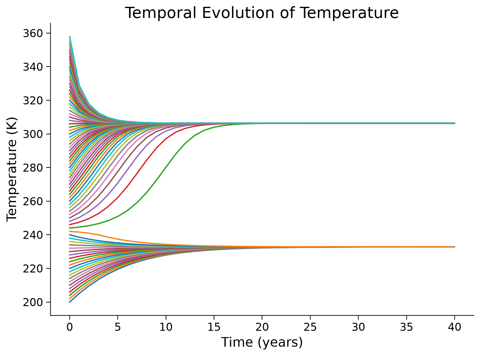
Let us explore how our model behaves under a variety of initial temperatures. We can use a for loop to compare different initial temperatures.
dt = 60.0 * 60.0 * 24.0 * 365.0  # time interval, one year expressed in seconds

fig, ax = plt.subplots()
for init_temp in T:  # suite of initial temperatures in K
    numtsteps = 40  #  number of years to run the model

    # for converting the number of seconds in a year
    sec_2_yr = 3.154e7

    # set the initial temperature (initial condition)
    T_series = [init_temp]

    # set the initial time to 0
    t_series = [0]

    # run the model
    for n in range(numtsteps):

        # calculate and append the time since running the model, dependent on dt and the numtsteps
        t_series.append((n + 1) * dt / sec_2_yr)

        # calculate and append the new temperature using our pre-defined function
        T_series.append(step_forward(T_series[n], tau=tau, Q=Q, dt=dt))

    # make plot
    ax.plot(t_series, T_series)

ax.set_title("Temporal Evolution of Temperature")
ax.set_xlabel("Time (years)")
ax.set_ylabel("Temperature (K)")
Text(0, 0.5, 'Temperature (K)')
Questions 1.2#
How many stable equilibria can you find on the figure above? Estimate their values.
What do these values represent on the figure you made in Part 1?
There is an unstable equilibrium state within this model. What is it’s value?
Submit your feedback#
Show code cell source
# @title Submit your feedback
content_review(f"{feedback_prefix}_Questions_1_2")
Section 1.3: Finding Equilibria Numerically & Determining Convergence or Divergence#
To verify the equilibrium solutions we identified graphically in the previous section, we can use python to find the exact values (i.e., where the rate of change in temperature is zero). That is find the temperatures that satisfy
To aid us, we will use brentq, a root-finding function from the scipy package.
# create function to find the forcing at the top of the atmosphere
def Ftoa(T):
    return ASR(Q, T) - OLR(tau, T)


#  brentq() requires a function and two end-points to be input as arguments
#  it will look for a root/zero of the function between those end-points
Teq1 = brentq(
    Ftoa, 200.0, 240.0
)  # these ranges are from the intersections of the graphs of ASR and OLR
Teq2 = brentq(Ftoa, 240.0, 280.0)
Teq3 = brentq(Ftoa, 280.0, 320.0)

print(Teq1, Teq2, Teq3)
232.77820135617048 242.83054107162232 306.3533415866786
To assess the stability of these equilibria, we can plot the difference in \(ASR\) and \(OSR\). This is the same function Ftoa that we calculated in the previous cell, but we will recalculate it below for plotting purposes.
# we've already calculated ASR and OLR above
fig, ax = plt.subplots()
F = ASR_vals - OLR_vals
ax.plot(T, F, color="k", linewidth=3)

# find positive values and fill with red
pos_ind1 = T <= Teq1
ax.fill_between(T[pos_ind1], 0, F[pos_ind1], color="red")

pos_ind2 = (T >= Teq2) & (T <= Teq3)
ax.fill_between(T[pos_ind2], 0, F[pos_ind2], color="red")

# find negative values and fill with blue
neg_ind1 = (T >= Teq1) & (T <= Teq2)
ax.fill_between(T[neg_ind1], 0, F[neg_ind1], color="blue")

neg_ind2 = T >= Teq3
ax.fill_between(T[neg_ind2], 0, F[neg_ind2], color="blue")

# plot vertical lines/names at equilibrium temperatures
ax.axvline(x=Teq1, color="k", ls=":")
ax.axvline(x=Teq2, color="k", ls=":")
ax.axvline(x=Teq3, color="k", ls=":")

ax.annotate(
    "$T_{eq1}$",
    xy=(Teq1 - 5, -295),
    xytext=(Teq1 - 5, -295),
    rotation=90,
    annotation_clip=False,
)
ax.annotate(
    "$T_{eq2}$",
    xy=(Teq2 - 5, -295),
    xytext=(Teq2 - 5, -295),
    rotation=90,
    annotation_clip=False,
)
ax.annotate(
    "$T_{eq3}$",
    xy=(Teq3 - 5, -295),
    xytext=(Teq3 - 5, -295),
    rotation=90,
    annotation_clip=False,
)

# plot arrows/text to show stability of equilibrium points
ax.annotate(
    "",
    xy=(232, -50),
    xytext=(200, -50),
    arrowprops=dict(facecolor="black", arrowstyle="-|>"),
)

ax.annotate(
    "",
    xy=(242.5, -50),
    xytext=(233, -50),
    arrowprops=dict(facecolor="black", arrowstyle="<|-"),
)

ax.annotate(
    "",
    xy=(305.5, -50),
    xytext=(243.5, -50),
    arrowprops=dict(facecolor="black", arrowstyle="-|>"),
)

ax.annotate(
    "",
    xy=(358, -50),
    xytext=(307, -50),
    arrowprops=dict(facecolor="black", arrowstyle="<|-"),
)


ax.annotate("convergence", xy=(358, -170), xytext=(307, -170), rotation=90)

ax.annotate("divergence", xy=(305.5, -170), xytext=(243.5, -170), rotation=90)

ax.annotate("convergence", xy=(242.5, -170), xytext=(233, -170), rotation=90)


ax.set_xlabel("Temperature (K)")
ax.set_ylabel("$ASR-OLR$ (Wm$^{-2}$)");
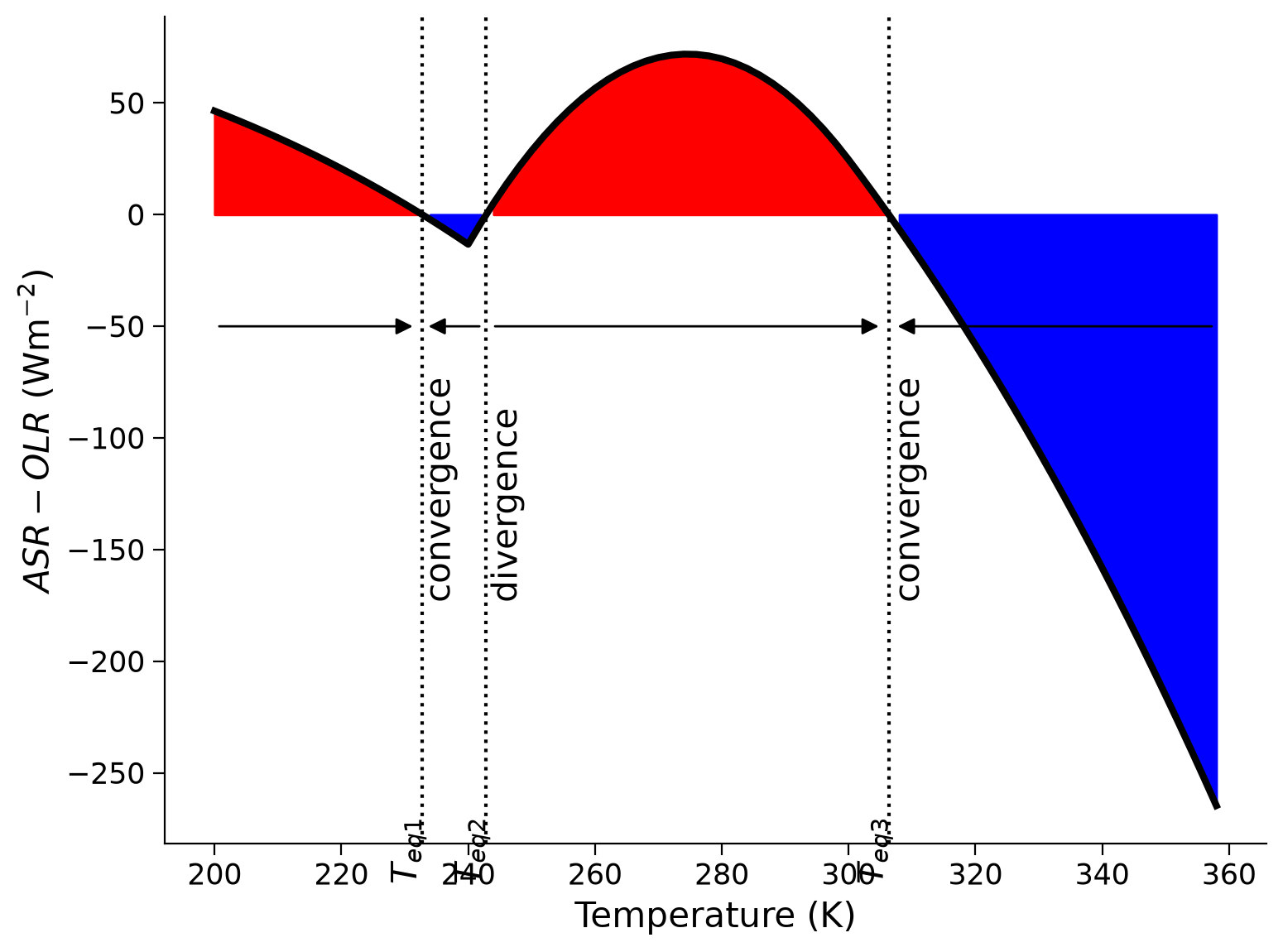
The red regions represent conditions where the Earth would warm, because the energy absorbed by the Earth system is greater than the energy emitted or reflected back into space.
The blue regions represent conditions where the Earth would cool, because the outgoing radiation is larger than the absorbed radiation.
For example, if Earth started at an initial temperature below \(T_{\text{eq1}}\) (in the left red region), it will move to the right on the \(x\)-axis, towards the \(T_{\text{eq1}}\) equilibrium state. Conversely, if Earth started between \(T_{\text{eq1}}\) and \(T_{\text{eq1}}\) (the left blue region), the temperature would decrease, moving left on the \(x\)-axis until it reaches \(T_{\text{eq1}}\). Thus \(T_{\text{eq1}}\) is a stable equilibrium as the temperature curves will tend to this point after a long time.
Questions 1.3#
Identify the stable and unstable equilibria from this graph. Do these agree with the figure you made in Section 1.2?
Submit your feedback#
Show code cell source
# @title Submit your feedback
content_review(f"{feedback_prefix}_Questions_1_3")
Section 2: Changing Insolation#
Section 2.1: Effect on the Number Equilibrium Solutions#
During Day 1 of this week, you learned that insolation (the amount of radiation Earth receives from the sun at the top of the atmosphere) fluctuates with time. Over Earth’s history, the insolation has sometimes been lower, and sometimes higher, than the currently observed \(340 \text{ Wm}^{-2}\).
These insolation changes directly affect the \(ASR\), causing Earth to warm or cool depending on whether it receives more or less insolation respectively. To look at the effect that changing insolation has on Earth’s equilibrium state(s), we can re-plot \(ASR\) as a function of temperature for several different insolation values (including the temperature-dependent albedo), alongside the \(OLR\).
# define the observed insolation
Q_vals = [220, 340, 420]  # W m^-2

fig, ax = plt.subplots()
for Q_2 in Q_vals:
    # calculate ASR and OLR for different values of T
    for tt, temp in enumerate(T):

        ASR_vals[tt] = ASR(Q_2, temp)

    # make plots
    ax.plot(T, ASR_vals, label="$ASR$ for $Q$ = " + str(Q_2) + " Wm$^{-2}$")

# note we calculated OLR previously, and it does not depend on Q
ax.plot(T, OLR_vals, label="$OLR$")


ax.set_xlabel("Temperature (K)")
ax.set_ylabel("Radiative Flux (Wm$^{-2}$)")
ax.legend()
<matplotlib.legend.Legend at 0x7f58444519d0>
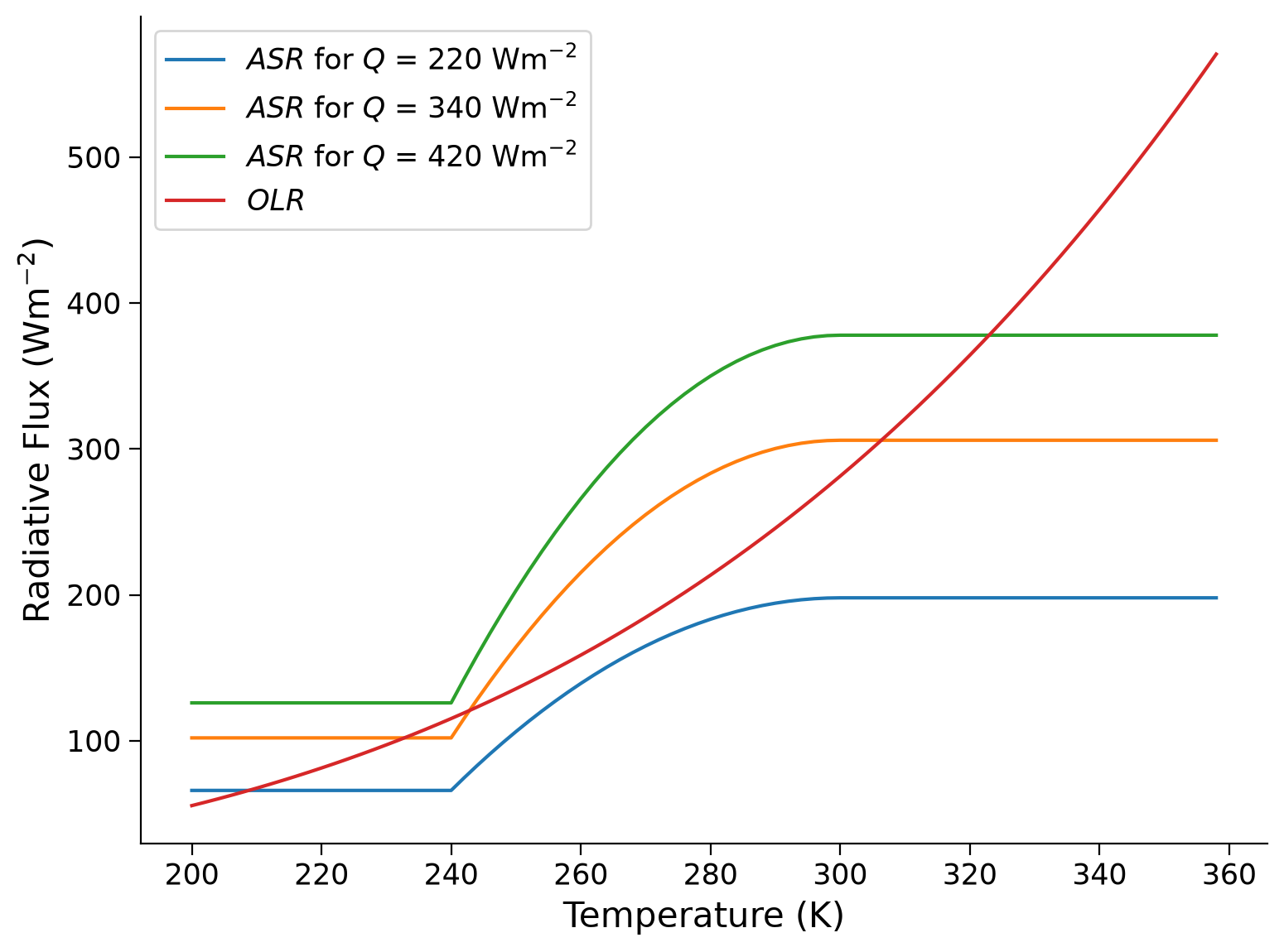
As we increase or decrease the insolation, the number of intersections between \(ASR\) and \(OLR\) can change! This means the number of equilibrium solutions for our model will also change.
Questions 2.1#
How many stable equilibrium solutions are there when \(Q=220 \text{ Wm}^{-2}\) ? Warm (ice-free) or cold (completely-frozen) state(s)?
For \(Q=420 \text{ Wm}^{-2}\) ? Warm or cold equilibrium state(s)?
Submit your feedback#
Show code cell source
# @title Submit your feedback
content_review(f"{feedback_prefix}_Questions_2_1")
Section 2.2: Effect on Equilibrium Temperatures#
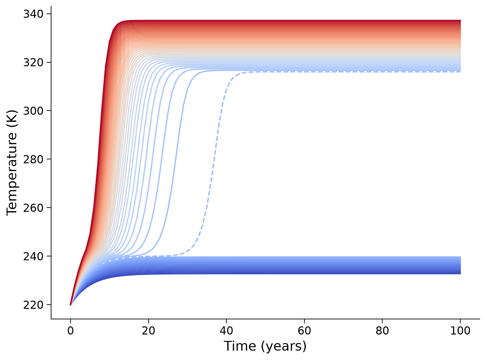
To understand how this effect translates to different equilibrium temperatures of our model over time, we will apply a range of insolation values to our model. Let us first start off with a very cold Earth, at \(220 \text{K}\), and warm the Earth by steadily increasing the insolation above our present-day \(340 \text{ Wm}^{-2}\) value.
# these are the values of insolation we will use
insolation_vals = np.arange(340, 500, 3)

# initial temperature we will use
init_temp = 220  # K

fig, ax = plt.subplots()

for i, insolation in enumerate(insolation_vals):  # suite of initial temperatures in K

    numtsteps = 100  #  number of years to run the model

    # for converting the number of seconds in a year
    sec_2_yr = 3.154e7

    # set the initial temperature (initial condition)
    T_series = [init_temp]

    # set the initial time to 0
    t_series = [0]

    # run the model
    for n in range(numtsteps):

        # calculate and append the time since running the model, dependent on dt and the numtsteps
        t_series.append((n + 1) * dt / sec_2_yr)

        # calculate and append the new temperature using our pre-defined function
        T_series.append(step_forward(T_series[n], tau=tau, Q=insolation, dt=dt))

    # make plot
    colors = plt.cm.coolwarm(np.linspace(0, 1, insolation_vals.shape[0]))
    if (
        insolation == 385
    ):  # This is just to highlight a particularly interesting insolation value
        ax.plot(t_series, T_series, color=colors[i], linestyle="dashed")
    else:
        ax.plot(t_series, T_series, color=colors[i])

ax.set_ylabel("Temperature (K)")
ax.set_xlabel("Time (years)")
Text(0.5, 0, 'Time (years)')
Questions 2.2: Climate Connection#
Noting the dashed blue lines, at approximately what temperature do you note a rapid transition from cold to warm equilibrium states? How do these compare to your equation for albedo?
How would you interpret the rapid transition in equilibrium temperatures with changing insolation (the big gap in the figure) using the \(ASR\) & \(OLR\) vs. temperature plot that you made in Section 2.1?
How does the time-varying behavior of the reddest (warm-state) lines relate to the ice-albedo feedback?
Submit your feedback#
Show code cell source
# @title Submit your feedback
content_review(f"{feedback_prefix}_Questions_2_2")
Summary#
In this tutorial, you learned about stable and unstable equilibria, identifying them from graphs and precisely calculating them. You also incorporated an ice-albedo feedback into your model to observe its effects on equilibrium solutions under varying insolation.
Resources#
Useful links:
The Climate Laboratory by Brian E. J. Rose