Tutorial 4: Oceanic Wind-Driven Circulation#

Week 1, Day 2: Ocean and Atmospheric Reanalysis

Content creators: Abigail Bodner

Content reviewers: Katrina Dobson, Danika Gupta, Maria Gonzalez, Will Gregory, Nahid Hasan, Paul Heubel, Sherry Mi, Beatriz Cosenza Muralles, Jenna Pearson, Chi Zhang, Ohad Zivan

Content editors: Paul Heubel, Brodie Pearson, Jenna Pearson, Chi Zhang, Ohad Zivan

Production editors: Wesley Banfield, Paul Heubel, Jenna Pearson, Konstantine Tsafatinos, Chi Zhang, Ohad Zivan

Our 2024 Sponsors: NFDI4Earth, CMIP

Tutorial Objectives#

Estimated timing of tutorial: 20 mins

The ocean’s motion is driven by radiation from the sun, winds, and various sources & sinks of fresh water (precipitation, rivers, melting and freezing ice). In the previous tutorial, you quantified the surface winds around the world. The surface winds drag on the surface of the ocean which results in water mass transport, known as Ekman transport.

In this tutorial you will use the ECCO (Estimating the Circulation and Climate of the Ocean) reanalysis data, to visualize the ocean’s surface currents and to compare these currents against local atmospheric conditions.

At the end of this tutorial, you will be able to

Access and manipulate ocean reanalysis data
Plot annual mean ocean surface currents and atmospheric surface winds
Compare oceanic and atmospheric circulation patterns

Setup#

# installations ( uncomment and run this cell ONLY when using google colab or kaggle )

# !pip install cartopy

import matplotlib.pyplot as plt
import os
import pooch
import tempfile
import xarray as xr
import warnings
from cartopy import crs as ccrs

#  suppress warnings issued by Cartopy when downloading data files
warnings.filterwarnings("ignore")

Install and import feedback gadget#

Helper functions#

Figure Settings#

Video 1: Ocean Wind-driven Circulation#

Submit your feedback#

If you want to download the slides: https://osf.io/download/f8c5r/

Submit your feedback#

Section 1: Load Ocean & Atmosphere Reanalysis Data#

Here you will load atmospheric near-surface winds (at 10-meter height), and then load the oceanic surface currents from ECCO reanalysis data.

Note, that each of these variables is a velocity with two components (zonal and meridional). These two velocity components must be loaded separately for each variable, so you will load four datasets.

Section 1.1: Exploring the Reanalysis Data#

Let’s examine the time (or temporal/output) frequency, which descibes the rate at which the reanalysis data is provided, for one of the ECCO variables (atm_wind_u).

Note that all the variables should have the same output frequency.

atm_wind_u.time

<xarray.DataArray 'time' (time: 12)> Size: 96B
array(['2016-01-16T12:00:00.000000000', '2016-02-15T12:00:00.000000000',
       '2016-03-16T12:00:00.000000000', '2016-04-16T00:00:00.000000000',
       '2016-05-16T12:00:00.000000000', '2016-06-16T00:00:00.000000000',
       '2016-07-16T12:00:00.000000000', '2016-08-16T12:00:00.000000000',
       '2016-09-16T00:00:00.000000000', '2016-10-16T12:00:00.000000000',
       '2016-11-16T00:00:00.000000000', '2016-12-16T12:00:00.000000000'],
      dtype='datetime64[ns]')
Coordinates:
  * time     (time) datetime64[ns] 96B 2016-01-16T12:00:00 ... 2016-12-16T12:...
Attributes:
    long_name:  center time of averaging period
    bounds:     time_bnds
    axis:       T

Questions 1.1#

Why do you think the atmospheric reanalysis dataset from the previous tutorial (ERA5) has higher output frequency (hourly) than the ECCO ocean reanalysis dataset (daily)?
What can you infer about the role of these two systems at different timescales in the climate system?

Click for solution

Submit your feedback#

Section 2: Plotting the Annual Mean of Global Surface Wind Stress#

In this section you will create global maps displaying the annual mean of atmospheric 10m winds.

First, you should compute the annual mean of the surface wind variables. You can do so by averaging over the time dimension using .mean(dim='time'). Since you have monthly data spanning only one year, .mean(dim='time') will give the annual mean for the year 2016.

You are now almost ready to plot!

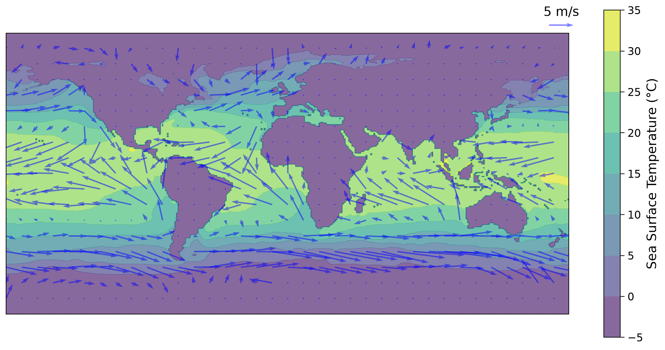
However, you currently have separate zonal and meridional wind velocity components \((u,v)\). An effective way of visualizing the total surface wind stress is to create a global map of the magnitude and direction of the wind velocity vector. This type of plot is known as a vector field. A vector is a special mathematical quantity that has both magnitude and direction, just like the wind! The velocity components describe the intensity of wind blowing in the zonal \(\left(u\right)\) or meridional \(\left(v\right)\) directions. Specifically, wind can blow eastward (positive \(u\)) or westward (negative \(u\)), as well as northward (positive \(v\)) or southward (negative \(v\)).

The total velocity vector is the vector sum of these two components and exhibits varying magnitude and direction. The magnitude \(\left(||u||\right)\) and direction \(\left(\varphi\right)\) of the total velocity vector can be determined using the following equations:

(3)#\[\begin{align} ||u|| = \sqrt{u^2 + v^2}, \ \ \ \ \varphi = \text{tan}^{-1}(\frac{v}{u}) \end{align}\]

When plotting a vector field using a computer, it is commonly referred to as a quiver plot. In our case, we will utilize a function created by Ryan Abernathey’s called quick_quiver() that calculates the magnitude and direction of the total velocity vector based on the given zonal and meridional components.

We will overlay the quiver plot on top of the annual mean ocean surface temperature (labeled here as theta).

# longitude ad latitude coordinates for plotting
lon = atm_wind_u_an_mean.longitude
lat = atm_wind_u_an_mean.latitude

# calculate magnitude of total velocity
mag = (atm_wind_u_an_mean**2 + atm_wind_v_an_mean**2) ** 0.5

# coarsen the grid so the arrows are distinguishable by only selecting
# some longitudes and latitudes defined by the last entry of the tuples.
slx = slice(None, None, 20)
sly = slice(None, None, 20)
sl2d = (slx, sly)

fig, ax = plt.subplots(
    figsize=(12, 6), subplot_kw={"projection": ccrs.Robinson(central_longitude=180)}
)

c = ax.contourf(lon, lat, ocn_surface_temp, alpha=0.65)

# plot quiver arrows indicating vector direction (winds are in blue, alpha is for opacity)
q = ax.quiver(
    lon[slx],
    lat[sly],
    atm_wind_u_an_mean[sl2d],
    atm_wind_v_an_mean[sl2d],
    color="b",
    alpha=0.5,
)

ax.quiverkey(q, 175, 95, 5, "5 m/s", coordinates="data")

fig.colorbar(c, label="Sea Surface Temperature (°C)")

<matplotlib.colorbar.Colorbar at 0x7f845dc909d0>

../../../_images/3ffe2db89a8d4b1305f14efbded049eb763142caad980db56648c899c8c54707.png

Section 3: Comparing Global Maps of Surface Currents and Winds#

In this section you will compute the annual mean of the ocean surface currents, similar to your above analyses of atmospheric winds, and you will create a global map that shows both of these variables simultaneously.

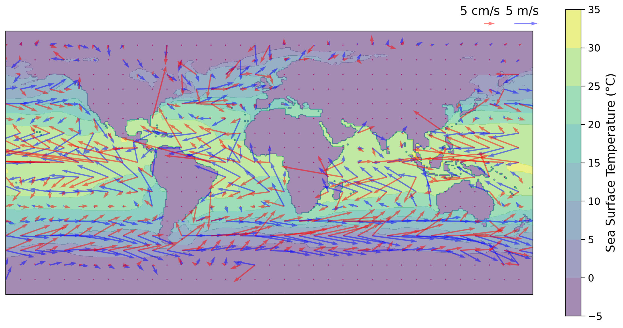
Let’s add ocean surface currents to the previous plot above, using red quivers. Note the scale of the arrows for the ocean and atmosphere are very different.

# longitude ad latitude coordinates for plotting
lon = atm_wind_u_an_mean.longitude
lat = atm_wind_u_an_mean.latitude

# calculate magnitude of total velocity
mag = (atm_wind_u_an_mean**2 + atm_wind_v_an_mean**2) ** 0.5

# coarsen the grid so the arrows are distinguishable by only selecting
# some longitudes and latitudes defined by slx and sly.
slx = slice(None, None, 20)
sly = slice(None, None, 20)
sl2d = (slx, sly)

# fig, ax = plt.subplots(**kwargs)
fig, ax = plt.subplots(
    figsize=(12, 6), subplot_kw={"projection": ccrs.Robinson(central_longitude=180)}
)

c = ax.contourf(lon, lat, ocn_surface_temp, alpha=0.5)

# plot quiver arrows indicating vector direction (winds are in blue, alpha is for opacity)
q1 = ax.quiver(
    lon[slx],
    lat[sly],
    atm_wind_u_an_mean[sl2d],
    atm_wind_v_an_mean[sl2d],
    color="b",
    alpha=0.5,
)

# plot quiver arrows indicating vector direction (ocean currents are in red, alpha is for opacity)
q2 = ax.quiver(
    lon[slx],
    lat[sly],
    ocn_surface_current_u_an_mean[sl2d],
    ocn_surface_current_v_an_mean[sl2d],
    color="r",
    alpha=0.5,
)

ax.quiverkey(q1, 175, 95, 5, "5 m/s  ", coordinates="data")

ax.quiverkey(q2, 150, 95, 0.05, "5 cm/s     ", coordinates="data")

fig.colorbar(c, label="Sea Surface Temperature (°C)")

<matplotlib.colorbar.Colorbar at 0x7f845c08cf10>

../../../_images/9f670c84860e45374e1f3b56d12074dcad8f0fc383fe33b2e1279e3a0b174ba7.png

Questions 3#

You may notice that the surface currents (red) are typically not aligned with the wind direction (blue). In fact, the surface ocean currents flow at an angle of approximately 45 degrees to the wind direction!

The combination of Coriolis force and the friction between ocean layers causes the wind-driven currents to turn and weaken with depth, eventually disappearing entirely at depth. The resulting current profile is called the Ekman Spiral, and the depth over which the spiral is present is called the Ekman layer. While the shape of this spiral can vary in time and space, the depth-integrated transport of water within the Ekman layer is called Ekman transport. Ekman transport is always 90 degrees to the right of the wind in the Northern Hemisphere, and 90 degrees to the left of the wind in the Southern Hemisphere. Under certain wind patterns or near coastlines, Ekman transport can lead to Ekman Pumping, where water is upwelled or downwelled depending on the wind direction. This process is particularly important for coastal ecosystems that rely on this upwelling (which is often seasonal) to bring nutrient-rich waters near the surface. These nutrients fuel the growth of tiny marine plants that support the entire food chain, upon which coastal economies often rely. These tiny plants are also responsible for most of the oxygen we breathe!

Do you observe a deflection of the surface currents relative to the wind?
Is this deflection the same in both the Northern and Southern Hemispheres?

Click for solution

Submit your feedback#

Summary#

In this tutorial, you explored how atmospheric winds can shape ocean surface currents.

You calculated the surface wind vector and assessed its influence on surface ocean currents called the wind-driven circulation.

This circulation influences global climate (e.g., moving heat between latitudes) and biogeochemical cycles (e.g., by driving upwelling of nutrient-rich water). In the next tutorial, you will explore another mechanism for ocean movement, density-driven circulation.

Resources#

Data for this tutorial can be accessed here.

Tutorial 4: Oceanic Wind-Driven Circulation

Contents

Tutorial 4: Oceanic Wind-Driven Circulation#

Tutorial Objectives#

Setup#

Install and import feedback gadget#

Helper functions#

Figure Settings#

Video 1: Ocean Wind-driven Circulation#

Submit your feedback#

Submit your feedback#

Section 1: Load Ocean & Atmosphere Reanalysis Data#

Section 1.1: Exploring the Reanalysis Data#

Questions 1.1#

Submit your feedback#

Section 2: Plotting the Annual Mean of Global Surface Wind Stress#

Section 3: Comparing Global Maps of Surface Currents and Winds#

Questions 3#

Submit your feedback#

Summary#

Resources#