


Tutorial 1: Calculating ENSO with Xarray#
Week 1, Day 2, Ocean-Atmosphere Reanalysis
Content creators: Abigail Bodner, Momme Hell, Aurora Basinski
Content reviewers: Yosemley Bermúdez, Katrina Dobson, Danika Gupta, Maria Gonzalez, Will Gregory, Nahid Hasan, Paul Heubel, Sherry Mi, Beatriz Cosenza Muralles, Jenna Pearson, Chi Zhang, Ohad Zivan
Content editors: Paul Heubel, Jenna Pearson, Chi Zhang, Ohad Zivan
Production editors: Wesley Banfield, Paul Heubel, Jenna Pearson, Konstantine Tsafatinos, Chi Zhang, Ohad Zivan
Our 2024 Sponsors: NFDI4Earth, CMIP
 #
#
Pythia credit: Rose, B. E. J., Kent, J., Tyle, K., Clyne, J., Banihirwe, A., Camron, D., May, R., Grover, M., Ford, R. R., Paul, K., Morley, J., Eroglu, O., Kailyn, L., & Zacharias, A. (2023). Pythia Foundations (Version v2023.05.01) https://zenodo.org/record/8065851
 #
#
Tutorial Objectives#
Estimated timing of tutorial: 30 mins
In this notebook (adapted from Project Pythia), you will practice using multiple tools to examine sea surface temperature (SST) and explore variations in the climate system that occur during El Niño and La Niña events. You will learn to:
Load sea surface temperature data from the CESM2 model
Mask data using
.where()Compute climatologies and anomalies using
.groupby()Use
.rolling()to compute moving averageCompute, normalize, and plot the Oceanic Niño Index
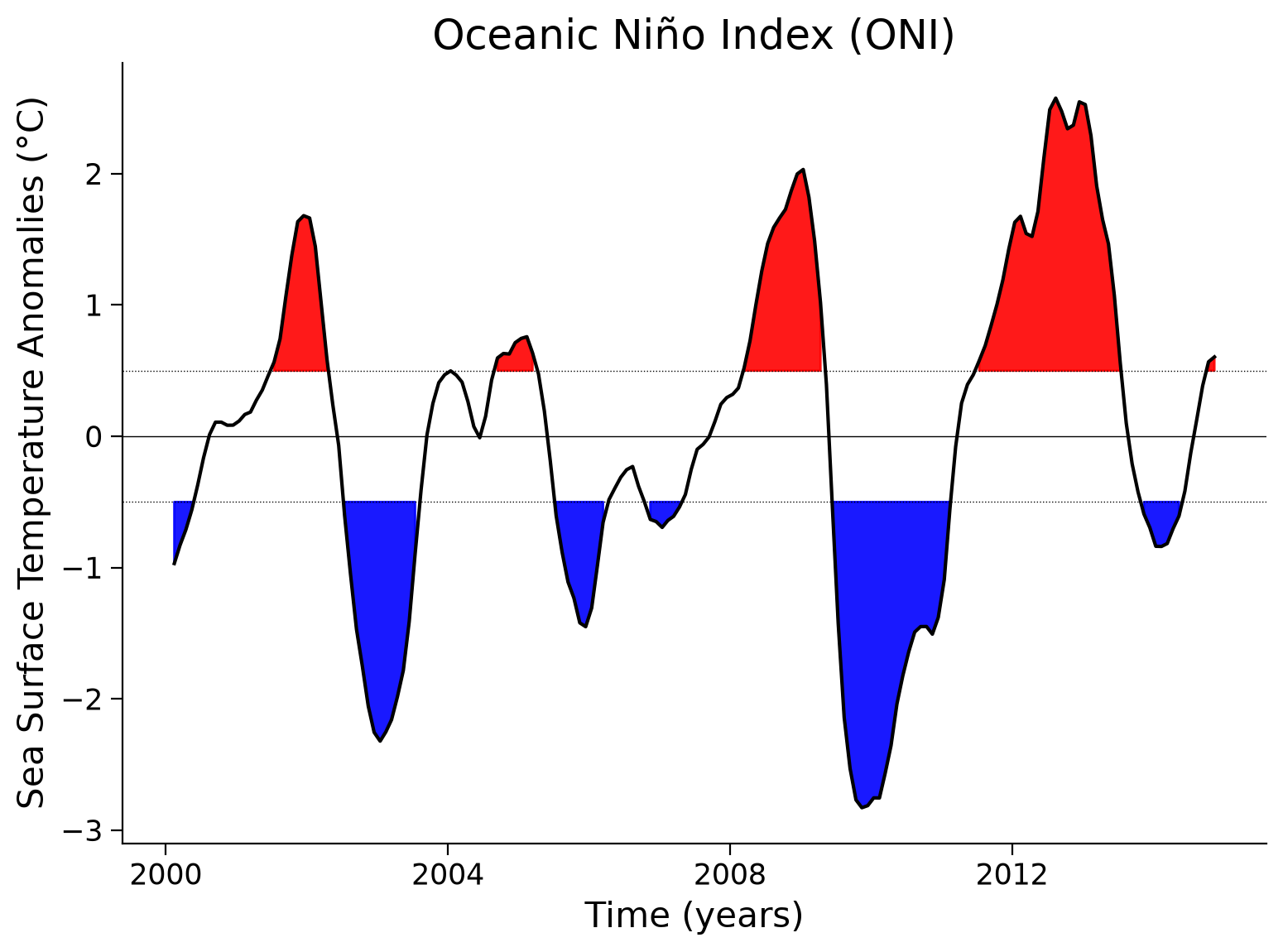
After completing the tasks above, you should be able to plot the Oceanic Niño Index that looks similar to the figure below. The red and blue regions correspond to the phases of El Niño and La Niña, respectively.
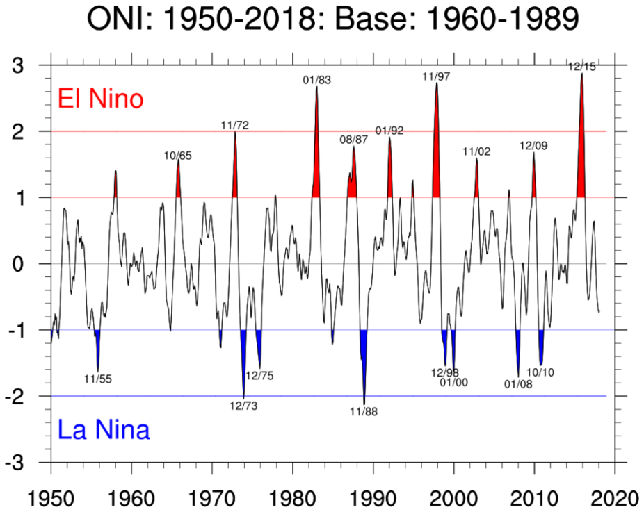
Credit: NCAR
Pythia credit: Rose, B. E. J., Kent, J., Tyle, K., Clyne, J., Banihirwe, A., Camron, D., May, R., Grover, M., Ford, R. R., Paul, K., Morley, J., Eroglu, O., Kailyn, L., & Zacharias, A. (2023). Pythia Foundations (Version v2023.05.01) https://zenodo.org/record/8065851
Setup#
# installations ( uncomment and run this cell ONLY when using google colab or kaggle )

# !pip install --upgrade --force-reinstall  pythia_datasets cartopy matplotlib geoviews xarray cftime nc-time-axis
# !pip install cartopy geoviews pythia_datasets
# # note you will need to restart the kernel after this - there should be a small button at the end of the output. Click 'Restart Session', then run the import cell and below.
# imports
import cartopy.crs as ccrs
import matplotlib.pyplot as plt
import xarray as xr
from pythia_datasets import DATASETS
import geoviews as gv
import geoviews.feature as gf
Install and import feedback gadget#
Show code cell source
# @title Install and import feedback gadget

!pip3 install vibecheck datatops --quiet

from vibecheck import DatatopsContentReviewContainer
def content_review(notebook_section: str):
    return DatatopsContentReviewContainer(
        "",  # No text prompt
        notebook_section,
        {
            "url": "https://pmyvdlilci.execute-api.us-east-1.amazonaws.com/klab",
            "name": "comptools_4clim",
            "user_key": "l5jpxuee",
        },
    ).render()


feedback_prefix = "W1D2_T1"
Figure Settings#
Show code cell source
# @title Figure Settings
import ipywidgets as widgets  # interactive display

%config InlineBackend.figure_format = 'retina'
plt.style.use(
    "https://raw.githubusercontent.com/neuromatch/climate-course-content/main/cma.mplstyle"
)
Video 1: El Niño Southern Oscillation#
Submit your feedback#
Show code cell source
# @title Submit your feedback
content_review(f"{feedback_prefix}_ENSO_Video")
If you want to download the slides: https://osf.io/download/t65v8/
Submit your feedback#
Show code cell source
# @title Submit your feedback
content_review(f"{feedback_prefix}_ENSO_Slides")
Section 1: Introduction to El Niño Southern Oscillation (ENSO)#
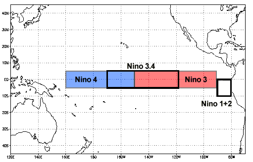
In W1D1 you practiced using Xarray to calculate a monthly climatology, climate anomalies, and a running average on monthly global Sea Surface Temperature (SST) data from the Community Earth System Model v2 (CESM2). You also used the .where() method to isolate SST data between 5ºN-5ºS and 190ºE-240ºE (or 170ºW-120ºW). This geographic region, known as the Niño 3.4 region, is in the tropical Pacific Ocean and is commonly used as a metric for determining the phase of the El Niño-Southern Oscillation (ENSO). ENSO is a recurring climate pattern involving changes in SST in the central and eastern tropical Pacific Ocean, which has two alternating phases:
El Niño: the phase of ENSO characterized by warmer than average SSTs in the central and eastern tropical Pacific Ocean, weakened east-to-west equatorial winds, and increased rainfall in the eastern tropical Pacific.
La Niña: the phase of ENSO which is characterized by cooler than average SSTs in the central and eastern tropical Pacific Ocean, stronger east-to-west equatorial winds, and decreased rainfall in the eastern tropical Pacific.
Section 1.1: Tropical Pacific Climate Processes#
To better understand the climate system processes that result in El Niño and La Niña events, let’s first consider typical climate conditions in the tropical Pacific Ocean. Recall from W1D1, trade winds are winds that blow east to west just north and south of the equator (these are sometimes referred to as “easterly” winds since the winds originate from the east and blow toward the west). As we discussed yesterday, the reason that the trade winds blow from east to west is related to Earth’s rotation, which causes the winds in the Northern Hemisphere to curve to the right and winds in the Southern Hemisphere to curve to the left. This is known as the Coriolis effect.
If Earth’s rotation affects air movement, do you think it also influences surface ocean water movement? It does! As trade winds blow across the tropical Pacific Ocean, they move water because of friction at the ocean surface. But because of the Coriolis effect, surface water moves to the right of the wind direction in the Northern Hemisphere and the left of the wind direction in the Southern Hemisphere, respectively. However, the speed and direction of water movement changes with depth. Ocean surface water moves at an angle to the wind, and the water under the surface water moves at a slightly larger angle, and the water below that turns at an even larger angle. The average direction of all this turning water is about a right angle from the wind direction. This average is known as Ekman transport. Since this process is driven by the trade winds, the strength of this ocean water transport varies in response to changes in the strength of the trade winds.
Section 1.2: Ocean-Atmosphere Interactions During El Niño and La Niña#
So, how does all of this relate to El Niño and La Niña? Changes in the strength of Pacific Ocean trade winds and the resulting impact on Ekman transport create variations in the tropical Pacific Ocean SST, which further results in changes to atmospheric circulation patterns and rainfall.
During an El Niño event, easterly trade winds are weaker. As a result, less warm surface water is transported to the west via Ekman transport, which causes a build-up of warm surface water in the eastern equatorial Pacific. This creates warmer-than-average SSTs in the eastern equatorial Pacific Ocean. The atmosphere responds to this warming with increased rising air motion and above-average rainfall in the eastern Pacific. In contrast, during a La Niña event, easterly trade winds are stronger. As a result, warmer surface water is transported to the west via Ekman transport, and cool water from deeper in the ocean rises in the eastern Pacific during a process known as upwelling. This creates cooler-than-average SSTs in the eastern equatorial Pacific Ocean. This cooling decreases rising air movement in the eastern Pacific, resulting in drier-than-average conditions.
In this tutorial, we’ll examine sea surface temperatures (SST) to explore variations in the climate system that occur during El Niño and La Niña events. Specifically, we will plot and interpret CESM2 SST data from the Niño 3.4 region.
This Niño 3.4 region is the most representative of the ENSO phenomenon (cf. Barnston et al. 1997) and therefore state-of-the-art. Regions 1 to 4 have been historical choices however are still used for historical comparisons and to investigate certain features of the multifaceted ENSO.
Section 2: Calculate the Oceanic Niño Index#
In this notebook, we are going to combine several topics and methods you’ve covered so far to compute the Oceanic Niño Index (ONI) using SST from the CESM2 submission to the CMIP6 project.
You will be working with CMIP6 data later in the week, particularly during W2D1. You can also learn more about CMIP, including additional methods to access CMIP data, please see our CMIP Resource Bank and the CMIP website.
To calculate the Oceanic Niño Index (ONI) you will:
Select SST data from Niño 3.4 region of 5ºN - 5ºS and 190ºE - 240ºE (or 170ºW - 120ºW) shown in the figure below.
Compute the climatology (here from 2000-2014) for the Niño 3.4 region.
Compute the monthly anomaly for the Niño 3.4 region.
Compute the area-weighted mean of the anomalies for the Niño 3.4 region to obtain a time series.
Smooth the time series of anomalies with a 3-month running mean.
Here we will briefly move through each of these steps, and tomorrow you will learn about them in more detail.
Section 2.1: Open the SST Data#
First, open the SST and areacello datasets, and use Xarray’s .merge() method to combine them into a single dataset:
# retrieve (fetch) the SST data we are going to be working on
SST_path = DATASETS.fetch("CESM2_sst_data.nc")

# open the file we acquired with xarray
SST_data = xr.open_dataset(SST_path)

# remember that a spatial cell of one times one degree does not have a constant area around the globe, each has a different size in square km.
# we need to account for this when taking averages for example

# fetch the weight for each grid cell
gridvars_path = DATASETS.fetch("CESM2_grid_variables.nc")

# open and save only the grid cell weights whose variable name is 'areacello'
# here the 'o' at the end refers to the area cells of the 'ocean' grid
areacello_data = xr.open_dataset(gridvars_path).areacello

# merge the SST and weights into one easy-to-use dataset - ds stands for dataset
ds_SST = xr.merge([SST_data, areacello_data])
ds_SST
/home/runner/micromamba/envs/climatematch/lib/python3.11/site-packages/xarray/conventions.py:440: SerializationWarning: variable 'tos' has multiple fill values {1e+20, 1e+20}, decoding all values to NaN.
  new_vars[k] = decode_cf_variable(
<xarray.Dataset> Size: 47MB
Dimensions:    (time: 180, d2: 2, lat: 180, lon: 360)
Coordinates:
  * time       (time) object 1kB 2000-01-15 12:00:00 ... 2014-12-15 12:00:00
  * lat        (lat) float64 1kB -89.5 -88.5 -87.5 -86.5 ... 86.5 87.5 88.5 89.5
  * lon        (lon) float64 3kB 0.5 1.5 2.5 3.5 4.5 ... 356.5 357.5 358.5 359.5
Dimensions without coordinates: d2
Data variables:
    time_bnds  (time, d2) object 3kB ...
    lat_bnds   (lat, d2) float64 3kB ...
    lon_bnds   (lon, d2) float64 6kB ...
    tos        (time, lat, lon) float32 47MB ...
    areacello  (lat, lon) float64 518kB ...
Attributes: (12/45)
    Conventions:            CF-1.7 CMIP-6.2
    activity_id:            CMIP
    branch_method:          standard
    branch_time_in_child:   674885.0
    branch_time_in_parent:  219000.0
    case_id:                972
    ...                     ...
    sub_experiment_id:      none
    table_id:               Omon
    tracking_id:            hdl:21.14100/2975ffd3-1d7b-47e3-961a-33f212ea4eb2
    variable_id:            tos
    variant_info:           CMIP6 20th century experiments (1850-2014) with C...
variant_label: r11i1p1f1Visualize the first time point in the early 2000s. You can check this on the indexes of the variable time from the ds_SST above. Note that using the .plot() function of our data array will automatically include this as a title when we select just the first time index.
# create a figure
fig = plt.figure()

# assign axis and define the projection -  centred in pacific
ax = plt.axes(projection=ccrs.Robinson(central_longitude=180))

# add coastlines
ax.coastlines()

# add gridlines (lon and lat)
ax.gridlines()

# plots the first time index (0) of SST (variable name 'tos') at the first time
ds_SST.tos.isel(time=0).plot(
    ax=ax,
    transform=ccrs.PlateCarree(),  # give our axis a map projection
    vmin=-2,
    vmax=30,          # define the temp range of the colorbar from -2 to 30C
    cmap="coolwarm",  # choose a colormap
)
<cartopy.mpl.geocollection.GeoQuadMesh at 0x7fa9c7f8a190>
/home/runner/micromamba/envs/climatematch/lib/python3.11/site-packages/cartopy/io/__init__.py:263: DownloadWarning: Downloading: https://naturalearth.s3.amazonaws.com/110m_physical/ne_110m_coastline.zip
  warnings.warn(f'Downloading: {url}', DownloadWarning)
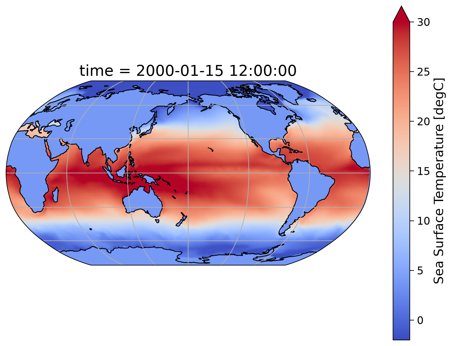
Click here for a description of the plot
A map plot showing the sea surface temperature (SST) in January 2000 ranging from -2°C to 30°C from the CESM Earth system model's historical simulation for the Sixth Phase of the Coupled Intercomparison Project (CMIP6). Equatorial regions show the warmest temperatures, and polar regions the lowest. A few larger patterns indicate that more than just the latitude is important to create the spatial SST distribution.Interactive Demo 2.1#
You can visualize what the next few times look like in the model by using the interactive sliderbar below.
# a bit more complicated code that allows interactive plots
gv.extension("bokeh")  # load Bokeh
dataset_plot = gv.Dataset(
    ds_SST.isel(time=slice(0, 10))
)  # slice only the first 10 timepoint, as it is a time consuming task
images = dataset_plot.to(gv.Image, ["longitude", "latitude"], "tos", "time")
images.opts(
    cmap="coolwarm",
    colorbar=True,
    width=600,
    height=400,
    projection=ccrs.Robinson(),
    clabel="Sea Surface Temperature [˚C]",
) * gf.coastline


---------------------------------------------------------------------------
KeyError                                  Traceback (most recent call last)
File ~/micromamba/envs/climatematch/lib/python3.11/site-packages/holoviews/core/dimension.py:1493, in Dimensioned._repr_mimebundle_(self, include, exclude)
   1486 def _repr_mimebundle_(self, include=None, exclude=None):
   1487     """Resolves the class hierarchy for the class rendering the
   1488     object using any display hooks registered on Store.display
   1489     hooks.  The output of all registered display_hooks is then
   1490     combined and returned.
   1491
   1492     """
-> 1493     return Store.render(self)

File ~/micromamba/envs/climatematch/lib/python3.11/site-packages/holoviews/core/options.py:1519, in Store.render(cls, obj)
   1517 data, metadata = {}, {}
   1518 for hook in hooks:
-> 1519     ret = hook(obj)
   1520     if ret is None:
   1521         continue

File ~/micromamba/envs/climatematch/lib/python3.11/site-packages/holoviews/ipython/display_hooks.py:330, in pprint_display(obj)
    328 if not ip.display_formatter.formatters["text/plain"].pprint:
    329     return None
--> 330 return display(obj, raw_output=True)

File ~/micromamba/envs/climatematch/lib/python3.11/site-packages/holoviews/ipython/display_hooks.py:304, in display(obj, raw_output, **kwargs)
    302 elif isinstance(obj, (HoloMap, DynamicMap)):
    303     with option_state(obj):
--> 304         output = map_display(obj)
    305 elif isinstance(obj, Plot):
    306     output = render(obj)

File ~/micromamba/envs/climatematch/lib/python3.11/site-packages/holoviews/ipython/display_hooks.py:193, in display_hook.<locals>.wrapped(element)
    191 try:
    192     max_frames = OutputSettings.options["max_frames"]
--> 193     mimebundle = fn(element, max_frames=max_frames)
    194     if mimebundle is None:
    195         return {}, {}

File ~/micromamba/envs/climatematch/lib/python3.11/site-packages/holoviews/ipython/display_hooks.py:246, in map_display(vmap, max_frames)
    243     max_frame_warning(max_frames)
    244     return None
--> 246 return render(vmap)

File ~/micromamba/envs/climatematch/lib/python3.11/site-packages/holoviews/ipython/display_hooks.py:62, in render(obj, **kwargs)
     59 if renderer.fig == "pdf":
     60     renderer = renderer.instance(fig="png")
---> 62 return renderer.components(obj, **kwargs)

File ~/micromamba/envs/climatematch/lib/python3.11/site-packages/holoviews/plotting/renderer.py:459, in Renderer.components(self, obj, fmt, comm, **kwargs)
    457 embed = not (dynamic or streams or self.widget_mode == "live") or config.embed
    458 if embed or config.comms == "default":
--> 459     return self._render_panel(plot, embed, comm)
    460 return self._render_ipywidget(plot)

File ~/micromamba/envs/climatematch/lib/python3.11/site-packages/holoviews/plotting/renderer.py:466, in Renderer._render_panel(self, plot, embed, comm)
    464 doc = Document()
    465 with config.set(embed=embed):
--> 466     model = plot.layout._render_model(doc, comm)
    467 if embed:
    468     return render_model(model, comm)

File ~/micromamba/envs/climatematch/lib/python3.11/site-packages/panel/viewable.py:803, in Viewable._render_model(self, doc, comm)
    801 if comm is None:
    802     comm = state._comm_manager.get_server_comm()
--> 803 model = self.get_root(doc, comm)
    805 if self._design and self._design.theme.bokeh_theme:
    806     doc.theme = self._design.theme.bokeh_theme

File ~/micromamba/envs/climatematch/lib/python3.11/site-packages/panel/layout/base.py:386, in Panel.get_root(self, doc, comm, preprocess)
    382 def get_root(
    383     self, doc: Document | None = None, comm: Comm | None = None,
    384     preprocess: bool = True
    385 ) -> Model:
--> 386     root = super().get_root(doc, comm, preprocess)
    387     # ALERT: Find a better way to handle this
    388     if hasattr(root, 'styles') and 'overflow-x' in root.styles:

File ~/micromamba/envs/climatematch/lib/python3.11/site-packages/panel/viewable.py:733, in Renderable.get_root(self, doc, comm, preprocess)
    731 wrapper = self._design._wrapper(self)
    732 if wrapper is self:
--> 733     root = self._get_model(doc, comm=comm)
    734     if preprocess:
    735         self._preprocess(root)

File ~/micromamba/envs/climatematch/lib/python3.11/site-packages/panel/layout/base.py:370, in Panel._get_model(self, doc, root, parent, comm)
    368 root = root or model
    369 self._models[root.ref['id']] = (model, parent)
--> 370 objects, _ = self._get_objects(model, [], doc, root, comm)
    371 props = self._get_properties(doc)
    372 props[self._property_mapping['objects']] = objects

File ~/micromamba/envs/climatematch/lib/python3.11/site-packages/panel/layout/base.py:352, in Panel._get_objects(self, model, old_objects, doc, root, comm)
    350 else:
    351     try:
--> 352         child = pane._get_model(doc, root, model, comm)
    353     except RerenderError as e:
    354         if e.layout is not None and e.layout is not self:

File ~/micromamba/envs/climatematch/lib/python3.11/site-packages/panel/pane/holoviews.py:494, in HoloViews._get_model(self, doc, root, parent, comm)
    492     plot = self.object
    493 else:
--> 494     plot = self._render(doc, comm, root)
    496 plot.pane = self
    497 backend = plot.renderer.backend

File ~/micromamba/envs/climatematch/lib/python3.11/site-packages/panel/pane/holoviews.py:588, in HoloViews._render(self, doc, comm, root)
    585     if comm:
    586         kwargs['comm'] = comm
--> 588 return renderer.get_plot(self.object, **kwargs)

File ~/micromamba/envs/climatematch/lib/python3.11/site-packages/holoviews/plotting/bokeh/renderer.py:77, in BokehRenderer.get_plot(self_or_cls, obj, doc, renderer, **kwargs)
     70 @bothmethod
     71 def get_plot(self_or_cls, obj, doc=None, renderer=None, **kwargs):
     72     """Given a HoloViews Viewable return a corresponding plot instance.
     73     Allows supplying a document attach the plot to, useful when
     74     combining the bokeh model with another plot.
     75
     76     """
---> 77     plot = super().get_plot(obj, doc, renderer, **kwargs)
     78     if plot.document is None:
     79         plot.document = Document() if self_or_cls.notebook_context else curdoc()

File ~/micromamba/envs/climatematch/lib/python3.11/site-packages/holoviews/plotting/renderer.py:300, in Renderer.get_plot(self_or_cls, obj, doc, renderer, comm, **kwargs)
    296     defaults = [kd.default for kd in plot.dimensions]
    297     init_key = tuple(
    298         v if d is None else d for v, d in zip(plot.keys[0], defaults, strict=None)
    299     )
--> 300     plot.update(init_key)
    301 else:
    302     plot = obj

File ~/micromamba/envs/climatematch/lib/python3.11/site-packages/holoviews/plotting/plot.py:1087, in DimensionedPlot.update(self, key)
   1085 if len(self) == 1 and key in (0, self.keys[0]) and not self.drawn:
   1086     return self.initialize_plot()
-> 1087 item = self.__getitem__(key)
   1088 self.traverse(lambda x: setattr(x, "_updated", True))
   1089 return item

File ~/micromamba/envs/climatematch/lib/python3.11/site-packages/holoviews/plotting/plot.py:503, in DimensionedPlot.__getitem__(self, frame)
    501     self.param.warning(f"Showing last frame available: {len(self)}")
    502 if not self.drawn:
--> 503     self.handles["fig"] = self.initialize_plot()
    504 if not isinstance(frame, tuple):
    505     frame = self.keys[frame]

File ~/micromamba/envs/climatematch/lib/python3.11/site-packages/geoviews/plotting/bokeh/plot.py:121, in GeoPlot.initialize_plot(self, ranges, plot, plots, source)
    119 def initialize_plot(self, ranges=None, plot=None, plots=None, source=None):
    120     opts = {} if isinstance(self, HvOverlayPlot) else {'source': source}
--> 121     fig = super().initialize_plot(ranges, plot, plots, **opts)
    122     style_element = self.current_frame.last if self.batched else self.current_frame
    123     el_ranges = match_spec(style_element, self.current_ranges) if self.current_ranges else {}

File ~/micromamba/envs/climatematch/lib/python3.11/site-packages/holoviews/plotting/bokeh/element.py:3906, in OverlayPlot.initialize_plot(self, ranges, plot, plots)
   3904 self.tabs = self.tabs or any(isinstance(sp, TablePlot) for sp in self.subplots.values())
   3905 if plot is None and not self.tabs and not self.batched:
-> 3906     plot = self._init_plot(key, element, ranges=ranges, plots=plots)
   3907     self._populate_axis_handles(plot)
   3908 self.handles["plot"] = plot

File ~/micromamba/envs/climatematch/lib/python3.11/site-packages/holoviews/plotting/bokeh/element.py:1150, in ElementPlot._init_plot(self, key, element, plots, ranges)
   1146 subplots = list(self.subplots.values()) if self.subplots else []
   1148 axis_specs = {"x": {}, "y": {}}
   1149 axis_specs["x"]["x"] = (
-> 1150     *self._axis_props(plots, subplots, element, ranges, pos=0),
   1151     self.xaxis,
   1152     {},
   1153 )
   1154 if self.multi_y and subplots:
   1155     if not BOKEH_GE_3_2_0:

File ~/micromamba/envs/climatematch/lib/python3.11/site-packages/holoviews/plotting/bokeh/element.py:936, in ElementPlot._axis_props(self, plots, subplots, element, ranges, pos, dim, range_tags_extras, extra_range_name)
    934 else:
    935     try:
--> 936         l, b, r, t = self.get_extents(range_el, ranges, dimension=dim)
    937     except TypeError:
    938         # Backward compatibility for e.g. GeoViews=<1.10.1 since dimension
    939         # is a newly added keyword argument in HoloViews 1.17
    940         l, b, r, t = self.get_extents(range_el, ranges)

File ~/micromamba/envs/climatematch/lib/python3.11/site-packages/geoviews/plotting/plot.py:64, in ProjectionPlot.get_extents(self, element, ranges, range_type, **kwargs)
     62     (x0, x1), (y0, y1) = proj.x_limits, proj.y_limits
     63     return (x0, y0, x1, y1)
---> 64 extents = super().get_extents(element, ranges, range_type)
     65 if not getattr(element, 'crs', None) or not self.geographic:
     66     return extents

File ~/micromamba/envs/climatematch/lib/python3.11/site-packages/holoviews/plotting/plot.py:2285, in GenericOverlayPlot.get_extents(self, overlay, ranges, range_type, dimension, **kwargs)
   2284 def get_extents(self, overlay, ranges, range_type="combined", dimension=None, **kwargs):
-> 2285     subplot_extents = self._get_subplot_extents(overlay, ranges, range_type, dimension)
   2286     zrange = isinstance(self.projection, str) and self.projection == "3d"
   2287     extents = {k: util.max_extents(rs, zrange) for k, rs in subplot_extents.items()}

File ~/micromamba/envs/climatematch/lib/python3.11/site-packages/holoviews/plotting/plot.py:2280, in GenericOverlayPlot._get_subplot_extents(self, overlay, ranges, range_type, dimension)
   2278         sp_ranges = util.match_spec(layer, ranges) if ranges else {}
   2279     for rt in extents:
-> 2280         extent = subplot.get_extents(layer, sp_ranges, range_type=rt)
   2281         extents[rt].append(extent)
   2282 return extents

File ~/micromamba/envs/climatematch/lib/python3.11/site-packages/geoviews/plotting/plot.py:70, in ProjectionPlot.get_extents(self, element, ranges, range_type, **kwargs)
     68     extents = None
     69 else:
---> 70     extents = project_extents(extents, element.crs, proj)
     71 return (np.nan,)*4 if not extents else extents

File ~/micromamba/envs/climatematch/lib/python3.11/site-packages/geoviews/util.py:72, in project_extents(extents, src_proj, dest_proj, tol)
     67 def project_extents(extents, src_proj, dest_proj, tol=1e-6):
     68     x1, y1, x2, y2 = extents
     70     if (isinstance(src_proj, ccrs.PlateCarree) and
     71         not isinstance(dest_proj, ccrs.PlateCarree) and
---> 72         src_proj.proj4_params['lon_0'] != 0):
     73         xoffset = src_proj.proj4_params['lon_0']
     74         x1 = x1 - xoffset

KeyError: 'lon_0'
:HoloMap   [time]
   :Overlay
      .Image.I     :Image   [lon,lat]   (Sea Surface Temperature)
      .Coastline.I :Feature   [Longitude,Latitude]
Click here for a description of the plot
An interactive map plot showing the sea surface temperature (SST) from January 2000 until October 2000 ranging from -2°C to 30°C from the CESM Earth system model's historical simulation for the Sixth Phase of the Coupled Intercomparison Project (CMIP6). Over the annual cycle, the warm and cold SST regions shift depending on the solar input. A few larger patterns indicate that more than just the latitude is important to create the spatial SST distribution, e.g. the equatorial pacific shows a cooler SST trench over the entire year compared to the surrounding subtropical waters.Section 2.2: Select the Niño 3.4 Region#
You may have noticed that the lon for the SST data is organized between 0°–360°E.
ds_SST.lon
<xarray.DataArray 'lon' (lon: 360)> Size: 3kB
array([  0.5,   1.5,   2.5, ..., 357.5, 358.5, 359.5])
Coordinates:
  * lon      (lon) float64 3kB 0.5 1.5 2.5 3.5 4.5 ... 356.5 357.5 358.5 359.5
Attributes:
    axis:           X
    bounds:         lon_bnds
    long_name:      longitude
    standard_name:  longitude
units: degrees_eastThis differs from how we typically use longitude (-180° to 180°). How do we convert the value of longitude between two systems (0° to 360° v.s. -180° to 180°)?
Let’s use lon2 to refer to the longitude system of 0° to 360° while lon refers to the system of -180° to 180°.
Note that 0° to 360° is equivalent to 0° to 180°, -180° to 0°.
In other words, lon2 = 181° is the same as lon = -179°. Hence, in the western hemisphere, lon2 = lon + 360.
Therefore, the Niño 3.4 region should be (-5° to 5°, 190° to 240°) using the lon2 system.
Now that we have identified the longitude values we need to select, there are a couple of ways to select the Niño 3.4 region. We will demonstrate how to use both below.
# select just the Niño 3.4 region (note our longitude values are in degrees east) by slicing
tos_nino34_op1 = ds_SST.sel(lat=slice(-5, 5), lon=slice(190, 240))
tos_nino34_op1
<xarray.Dataset> Size: 370kB
Dimensions:    (time: 180, d2: 2, lat: 10, lon: 50)
Coordinates:
  * time       (time) object 1kB 2000-01-15 12:00:00 ... 2014-12-15 12:00:00
  * lat        (lat) float64 80B -4.5 -3.5 -2.5 -1.5 -0.5 0.5 1.5 2.5 3.5 4.5
  * lon        (lon) float64 400B 190.5 191.5 192.5 193.5 ... 237.5 238.5 239.5
Dimensions without coordinates: d2
Data variables:
    time_bnds  (time, d2) object 3kB ...
    lat_bnds   (lat, d2) float64 160B ...
    lon_bnds   (lon, d2) float64 800B ...
    tos        (time, lat, lon) float32 360kB ...
    areacello  (lat, lon) float64 4kB ...
Attributes: (12/45)
    Conventions:            CF-1.7 CMIP-6.2
    activity_id:            CMIP
    branch_method:          standard
    branch_time_in_child:   674885.0
    branch_time_in_parent:  219000.0
    case_id:                972
    ...                     ...
    sub_experiment_id:      none
    table_id:               Omon
    tracking_id:            hdl:21.14100/2975ffd3-1d7b-47e3-961a-33f212ea4eb2
    variable_id:            tos
    variant_info:           CMIP6 20th century experiments (1850-2014) with C...
variant_label: r11i1p1f1Use
.where()and select all values within the bounds of interest
# select just the Niño 3.4 region (note our longitude values are in degrees east) by boolean conditioning
tos_nino34_op2 = ds_SST.where(
    (ds_SST.lat > -5) & (ds_SST.lat < 5) & (ds_SST.lon > 190) & (ds_SST.lon < 240),
    drop=True,
)  # use dataset .where() function. use boolean commands. drop data that is not of interest
tos_nino34_op2
<xarray.Dataset> Size: 2MB
Dimensions:    (time: 180, d2: 2, lat: 10, lon: 50)
Coordinates:
  * time       (time) object 1kB 2000-01-15 12:00:00 ... 2014-12-15 12:00:00
  * lat        (lat) float64 80B -4.5 -3.5 -2.5 -1.5 -0.5 0.5 1.5 2.5 3.5 4.5
  * lon        (lon) float64 400B 190.5 191.5 192.5 193.5 ... 237.5 238.5 239.5
Dimensions without coordinates: d2
Data variables:
    time_bnds  (time, d2, lat, lon) object 1MB 2000-01-01 00:00:00 ... 2015-0...
    lat_bnds   (lat, d2, lon) float64 8kB -5.0 -5.0 -5.0 -5.0 ... 5.0 5.0 5.0
    lon_bnds   (lon, d2, lat) float64 8kB 190.0 190.0 190.0 ... 240.0 240.0
    tos        (time, lat, lon) float32 360kB 28.26 28.16 28.06 ... 28.57 28.63
    areacello  (lat, lon) float64 4kB 1.233e+10 1.233e+10 ... 1.233e+10
Attributes: (12/45)
    Conventions:            CF-1.7 CMIP-6.2
    activity_id:            CMIP
    branch_method:          standard
    branch_time_in_child:   674885.0
    branch_time_in_parent:  219000.0
    case_id:                972
    ...                     ...
    sub_experiment_id:      none
    table_id:               Omon
    tracking_id:            hdl:21.14100/2975ffd3-1d7b-47e3-961a-33f212ea4eb2
    variable_id:            tos
    variant_info:           CMIP6 20th century experiments (1850-2014) with C...
variant_label: r11i1p1f1You can verify that tos_nino34_op1 and tos_nino34_op2 are the same by comparing the lat and lon indexes.
We only need one of these, so let us choose the second option and set that to the variable we will use moving forward.
# SST in just the Niño 3.4 region
tos_nino34 = tos_nino34_op2
Let’s utilize the same code we used to plot the entire Earth, but this time focusing on the Niño 3.4 region slice only.
# define the figure size
fig = plt.figure(constrained_layout=True)

# assign axis and projection
ax = plt.axes(projection=ccrs.Robinson(central_longitude=180))

# add coastlines
ax.coastlines()

# add gridlines (lon and lat)
ax.gridlines()

# plot as above
tos_nino34.tos.isel(time=0).plot(
    ax=ax, transform=ccrs.PlateCarree(), vmin=-2, vmax=30, cmap="coolwarm"
)

# make sure we see more areas of the earth and not only the square around Niño 3.4
ax.set_extent((120, 300, 10, -10))
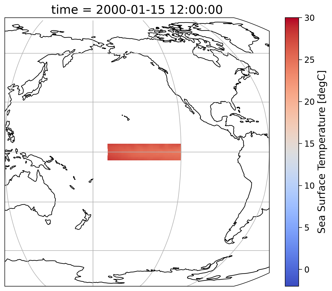
Click here for a description of the plot
A map plot zoomed into the Pacific Ocean showing the sea surface temperature (SST) in the Niño3.4 region in January 2000 ranging from -2°C to 30°C from the CESM Earth system models historical simulation for the Sixth Phase of the Coupled Intercomparison Project (CMIP6). The closer to the equator, the colder the water masses at the surface caused by upwelling from below induced by easterly winds and consequent Ekman transport.Interactive Demo 2.2#
Below we plot an interactive version of the Niño 3.4 region. You can explore the data by zooming in with the tools from the righthand toolbar and visualize what the next few time steps look like in the model by using the interactive slider bar on the most right. Note that the color bar and the corresponding SST scale have changed to make the changing pattern more visible.
# again more complicated code that allows interactive plots
gv.extension("bokeh")  # load Bokeh
dataset_plot = gv.Dataset(
    ds_SST.where(
    (ds_SST.lat > -5) & (ds_SST.lat < 5) & (ds_SST.lon > 190) & (ds_SST.lon < 240)
).isel(time=slice(0, 10))
)  # slice only the first 10 timepoint, as it is a time consuming task
images = dataset_plot.to(gv.Image, ["longitude", "latitude"], "tos", "time")
# aesthetics
images.opts(
    cmap="coolwarm",
    colorbar=True,
    width=600,
    height=400,
    projection=ccrs.Robinson(central_longitude=180),
    clabel="Sea Surface Temperature [˚C]",
) * gf.coastline
---------------------------------------------------------------------------
KeyError                                  Traceback (most recent call last)
File ~/micromamba/envs/climatematch/lib/python3.11/site-packages/holoviews/core/dimension.py:1493, in Dimensioned._repr_mimebundle_(self, include, exclude)
   1486 def _repr_mimebundle_(self, include=None, exclude=None):
   1487     """Resolves the class hierarchy for the class rendering the
   1488     object using any display hooks registered on Store.display
   1489     hooks.  The output of all registered display_hooks is then
   1490     combined and returned.
   1491
   1492     """
-> 1493     return Store.render(self)

File ~/micromamba/envs/climatematch/lib/python3.11/site-packages/holoviews/core/options.py:1519, in Store.render(cls, obj)
   1517 data, metadata = {}, {}
   1518 for hook in hooks:
-> 1519     ret = hook(obj)
   1520     if ret is None:
   1521         continue

File ~/micromamba/envs/climatematch/lib/python3.11/site-packages/holoviews/ipython/display_hooks.py:330, in pprint_display(obj)
    328 if not ip.display_formatter.formatters["text/plain"].pprint:
    329     return None
--> 330 return display(obj, raw_output=True)

File ~/micromamba/envs/climatematch/lib/python3.11/site-packages/holoviews/ipython/display_hooks.py:304, in display(obj, raw_output, **kwargs)
    302 elif isinstance(obj, (HoloMap, DynamicMap)):
    303     with option_state(obj):
--> 304         output = map_display(obj)
    305 elif isinstance(obj, Plot):
    306     output = render(obj)

File ~/micromamba/envs/climatematch/lib/python3.11/site-packages/holoviews/ipython/display_hooks.py:193, in display_hook.<locals>.wrapped(element)
    191 try:
    192     max_frames = OutputSettings.options["max_frames"]
--> 193     mimebundle = fn(element, max_frames=max_frames)
    194     if mimebundle is None:
    195         return {}, {}

File ~/micromamba/envs/climatematch/lib/python3.11/site-packages/holoviews/ipython/display_hooks.py:246, in map_display(vmap, max_frames)
    243     max_frame_warning(max_frames)
    244     return None
--> 246 return render(vmap)

File ~/micromamba/envs/climatematch/lib/python3.11/site-packages/holoviews/ipython/display_hooks.py:62, in render(obj, **kwargs)
     59 if renderer.fig == "pdf":
     60     renderer = renderer.instance(fig="png")
---> 62 return renderer.components(obj, **kwargs)

File ~/micromamba/envs/climatematch/lib/python3.11/site-packages/holoviews/plotting/renderer.py:459, in Renderer.components(self, obj, fmt, comm, **kwargs)
    457 embed = not (dynamic or streams or self.widget_mode == "live") or config.embed
    458 if embed or config.comms == "default":
--> 459     return self._render_panel(plot, embed, comm)
    460 return self._render_ipywidget(plot)

File ~/micromamba/envs/climatematch/lib/python3.11/site-packages/holoviews/plotting/renderer.py:466, in Renderer._render_panel(self, plot, embed, comm)
    464 doc = Document()
    465 with config.set(embed=embed):
--> 466     model = plot.layout._render_model(doc, comm)
    467 if embed:
    468     return render_model(model, comm)

File ~/micromamba/envs/climatematch/lib/python3.11/site-packages/panel/viewable.py:803, in Viewable._render_model(self, doc, comm)
    801 if comm is None:
    802     comm = state._comm_manager.get_server_comm()
--> 803 model = self.get_root(doc, comm)
    805 if self._design and self._design.theme.bokeh_theme:
    806     doc.theme = self._design.theme.bokeh_theme

File ~/micromamba/envs/climatematch/lib/python3.11/site-packages/panel/layout/base.py:386, in Panel.get_root(self, doc, comm, preprocess)
    382 def get_root(
    383     self, doc: Document | None = None, comm: Comm | None = None,
    384     preprocess: bool = True
    385 ) -> Model:
--> 386     root = super().get_root(doc, comm, preprocess)
    387     # ALERT: Find a better way to handle this
    388     if hasattr(root, 'styles') and 'overflow-x' in root.styles:

File ~/micromamba/envs/climatematch/lib/python3.11/site-packages/panel/viewable.py:733, in Renderable.get_root(self, doc, comm, preprocess)
    731 wrapper = self._design._wrapper(self)
    732 if wrapper is self:
--> 733     root = self._get_model(doc, comm=comm)
    734     if preprocess:
    735         self._preprocess(root)

File ~/micromamba/envs/climatematch/lib/python3.11/site-packages/panel/layout/base.py:370, in Panel._get_model(self, doc, root, parent, comm)
    368 root = root or model
    369 self._models[root.ref['id']] = (model, parent)
--> 370 objects, _ = self._get_objects(model, [], doc, root, comm)
    371 props = self._get_properties(doc)
    372 props[self._property_mapping['objects']] = objects

File ~/micromamba/envs/climatematch/lib/python3.11/site-packages/panel/layout/base.py:352, in Panel._get_objects(self, model, old_objects, doc, root, comm)
    350 else:
    351     try:
--> 352         child = pane._get_model(doc, root, model, comm)
    353     except RerenderError as e:
    354         if e.layout is not None and e.layout is not self:

File ~/micromamba/envs/climatematch/lib/python3.11/site-packages/panel/pane/holoviews.py:494, in HoloViews._get_model(self, doc, root, parent, comm)
    492     plot = self.object
    493 else:
--> 494     plot = self._render(doc, comm, root)
    496 plot.pane = self
    497 backend = plot.renderer.backend

File ~/micromamba/envs/climatematch/lib/python3.11/site-packages/panel/pane/holoviews.py:588, in HoloViews._render(self, doc, comm, root)
    585     if comm:
    586         kwargs['comm'] = comm
--> 588 return renderer.get_plot(self.object, **kwargs)

File ~/micromamba/envs/climatematch/lib/python3.11/site-packages/holoviews/plotting/bokeh/renderer.py:77, in BokehRenderer.get_plot(self_or_cls, obj, doc, renderer, **kwargs)
     70 @bothmethod
     71 def get_plot(self_or_cls, obj, doc=None, renderer=None, **kwargs):
     72     """Given a HoloViews Viewable return a corresponding plot instance.
     73     Allows supplying a document attach the plot to, useful when
     74     combining the bokeh model with another plot.
     75
     76     """
---> 77     plot = super().get_plot(obj, doc, renderer, **kwargs)
     78     if plot.document is None:
     79         plot.document = Document() if self_or_cls.notebook_context else curdoc()

File ~/micromamba/envs/climatematch/lib/python3.11/site-packages/holoviews/plotting/renderer.py:300, in Renderer.get_plot(self_or_cls, obj, doc, renderer, comm, **kwargs)
    296     defaults = [kd.default for kd in plot.dimensions]
    297     init_key = tuple(
    298         v if d is None else d for v, d in zip(plot.keys[0], defaults, strict=None)
    299     )
--> 300     plot.update(init_key)
    301 else:
    302     plot = obj

File ~/micromamba/envs/climatematch/lib/python3.11/site-packages/holoviews/plotting/plot.py:1087, in DimensionedPlot.update(self, key)
   1085 if len(self) == 1 and key in (0, self.keys[0]) and not self.drawn:
   1086     return self.initialize_plot()
-> 1087 item = self.__getitem__(key)
   1088 self.traverse(lambda x: setattr(x, "_updated", True))
   1089 return item

File ~/micromamba/envs/climatematch/lib/python3.11/site-packages/holoviews/plotting/plot.py:503, in DimensionedPlot.__getitem__(self, frame)
    501     self.param.warning(f"Showing last frame available: {len(self)}")
    502 if not self.drawn:
--> 503     self.handles["fig"] = self.initialize_plot()
    504 if not isinstance(frame, tuple):
    505     frame = self.keys[frame]

File ~/micromamba/envs/climatematch/lib/python3.11/site-packages/geoviews/plotting/bokeh/plot.py:121, in GeoPlot.initialize_plot(self, ranges, plot, plots, source)
    119 def initialize_plot(self, ranges=None, plot=None, plots=None, source=None):
    120     opts = {} if isinstance(self, HvOverlayPlot) else {'source': source}
--> 121     fig = super().initialize_plot(ranges, plot, plots, **opts)
    122     style_element = self.current_frame.last if self.batched else self.current_frame
    123     el_ranges = match_spec(style_element, self.current_ranges) if self.current_ranges else {}

File ~/micromamba/envs/climatematch/lib/python3.11/site-packages/holoviews/plotting/bokeh/element.py:3906, in OverlayPlot.initialize_plot(self, ranges, plot, plots)
   3904 self.tabs = self.tabs or any(isinstance(sp, TablePlot) for sp in self.subplots.values())
   3905 if plot is None and not self.tabs and not self.batched:
-> 3906     plot = self._init_plot(key, element, ranges=ranges, plots=plots)
   3907     self._populate_axis_handles(plot)
   3908 self.handles["plot"] = plot

File ~/micromamba/envs/climatematch/lib/python3.11/site-packages/holoviews/plotting/bokeh/element.py:1150, in ElementPlot._init_plot(self, key, element, plots, ranges)
   1146 subplots = list(self.subplots.values()) if self.subplots else []
   1148 axis_specs = {"x": {}, "y": {}}
   1149 axis_specs["x"]["x"] = (
-> 1150     *self._axis_props(plots, subplots, element, ranges, pos=0),
   1151     self.xaxis,
   1152     {},
   1153 )
   1154 if self.multi_y and subplots:
   1155     if not BOKEH_GE_3_2_0:

File ~/micromamba/envs/climatematch/lib/python3.11/site-packages/holoviews/plotting/bokeh/element.py:936, in ElementPlot._axis_props(self, plots, subplots, element, ranges, pos, dim, range_tags_extras, extra_range_name)
    934 else:
    935     try:
--> 936         l, b, r, t = self.get_extents(range_el, ranges, dimension=dim)
    937     except TypeError:
    938         # Backward compatibility for e.g. GeoViews=<1.10.1 since dimension
    939         # is a newly added keyword argument in HoloViews 1.17
    940         l, b, r, t = self.get_extents(range_el, ranges)

File ~/micromamba/envs/climatematch/lib/python3.11/site-packages/geoviews/plotting/plot.py:64, in ProjectionPlot.get_extents(self, element, ranges, range_type, **kwargs)
     62     (x0, x1), (y0, y1) = proj.x_limits, proj.y_limits
     63     return (x0, y0, x1, y1)
---> 64 extents = super().get_extents(element, ranges, range_type)
     65 if not getattr(element, 'crs', None) or not self.geographic:
     66     return extents

File ~/micromamba/envs/climatematch/lib/python3.11/site-packages/holoviews/plotting/plot.py:2285, in GenericOverlayPlot.get_extents(self, overlay, ranges, range_type, dimension, **kwargs)
   2284 def get_extents(self, overlay, ranges, range_type="combined", dimension=None, **kwargs):
-> 2285     subplot_extents = self._get_subplot_extents(overlay, ranges, range_type, dimension)
   2286     zrange = isinstance(self.projection, str) and self.projection == "3d"
   2287     extents = {k: util.max_extents(rs, zrange) for k, rs in subplot_extents.items()}

File ~/micromamba/envs/climatematch/lib/python3.11/site-packages/holoviews/plotting/plot.py:2280, in GenericOverlayPlot._get_subplot_extents(self, overlay, ranges, range_type, dimension)
   2278         sp_ranges = util.match_spec(layer, ranges) if ranges else {}
   2279     for rt in extents:
-> 2280         extent = subplot.get_extents(layer, sp_ranges, range_type=rt)
   2281         extents[rt].append(extent)
   2282 return extents

File ~/micromamba/envs/climatematch/lib/python3.11/site-packages/geoviews/plotting/plot.py:70, in ProjectionPlot.get_extents(self, element, ranges, range_type, **kwargs)
     68     extents = None
     69 else:
---> 70     extents = project_extents(extents, element.crs, proj)
     71 return (np.nan,)*4 if not extents else extents

File ~/micromamba/envs/climatematch/lib/python3.11/site-packages/geoviews/util.py:72, in project_extents(extents, src_proj, dest_proj, tol)
     67 def project_extents(extents, src_proj, dest_proj, tol=1e-6):
     68     x1, y1, x2, y2 = extents
     70     if (isinstance(src_proj, ccrs.PlateCarree) and
     71         not isinstance(dest_proj, ccrs.PlateCarree) and
---> 72         src_proj.proj4_params['lon_0'] != 0):
     73         xoffset = src_proj.proj4_params['lon_0']
     74         x1 = x1 - xoffset

KeyError: 'lon_0'
:HoloMap   [time]
   :Overlay
      .Image.I     :Image   [lon,lat]   (Sea Surface Temperature)
      .Coastline.I :Feature   [Longitude,Latitude]
Click here for a description of the plot
An interactive map plot showing the sea surface temperature (SST) from January 2000 until October 2000 ranging from 23.5°C to 30.5°C from the CESM Earth system model's historical simulation for the Sixth Phase of the Coupled Intercomparison Project (CMIP6). Over the annual cycle, the SST increases in the northern hemispherical summer. The closer to the equator, the colder the water masses at the surface caused by upwelling induced by easterly winds and consequent Ekman transport. The more west in the region the warmer the water masses also caused by this transport.Section 2.3: Compute the Climatology and Anomalies#
Now that we have selected our area, we can compute the monthly anomaly by first grouping all the data by month, and then subtracting the monthly climatology from each month. Taking the area-weighted average of these anomalies finally results in a time series with a temporal resolution of months.
# group the dataset by month
tos_nino34_mon = tos_nino34.tos.groupby("time.month")

# find the monthly climatology in the Nino 3.4 region
tos_nino34_clim = tos_nino34_mon.mean(dim="time")

# find the monthly anomaly in the Nino 3.4 region
tos_nino34_anom = tos_nino34_mon - tos_nino34_clim

# take the area-weighted average of anomalies in the Nino 3.4 region
tos_nino34_anom_mean = tos_nino34_anom.weighted(tos_nino34.areacello).mean(
    dim=["lat", "lon"]
)
tos_nino34_anom_mean
<xarray.DataArray 'tos' (time: 180)> Size: 1kB
array([-1.09020298, -0.9468297 , -0.87016873, -0.67314577, -0.58964466,
       -0.42163336, -0.1045906 ,  0.03671593,  0.10723417,  0.1785215 ,
        0.03699054,  0.03701807,  0.18047597,  0.13209798,  0.18591613,
        0.23601162,  0.40335289,  0.41607814,  0.56452046,  0.71568725,
        0.94604373,  1.54824446,  1.64511477,  1.71039075,  1.68536357,
        1.59079582,  1.06137082,  0.42683043,  0.28220144,  0.01182273,
       -0.50274312, -1.31489684, -1.34690005, -1.74364303, -2.16279013,
       -2.25649883, -2.34426792, -2.36370231, -2.04569941, -2.06573345,
       -1.83853617, -1.44441816, -0.95012921, -0.29584981,  0.02383253,
        0.30428055,  0.42201289,  0.49855485,  0.48539398,  0.51069792,
        0.39988403,  0.32679854,  0.06415631, -0.1690822 ,  0.07204664,
        0.55496829,  0.65673471,  0.57821735,  0.65645905,  0.64569503,
        0.83701738,  0.7530504 ,  0.68472185,  0.46625658,  0.27632614,
       -0.163     , -0.6672963 , -0.97958275, -1.00201312, -1.347174  ,
       -1.345642  , -1.56877078, -1.43570677, -0.91709918, -0.60461377,
       -0.44474807, -0.39675864, -0.34406608, -0.19599503, -0.22287632,
       -0.27117907, -0.64625189, -0.58092371, -0.6721508 , -0.69564099,
       -0.71416744, -0.51178688, -0.6025152 , -0.50095787, -0.22583469,
       -0.02674857, -0.04463511, -0.11126006,  0.14102331,  0.30948337,
        0.28171976,  0.29325427,  0.38412102,  0.42648502,  0.75224686,
        1.00070399,  1.25250362,  1.52579139,  1.62650826,  1.62089055,
        1.74093498,  1.82211026,  2.04950708,  2.12185872,  1.92467518,
        1.41653594,  1.11950452,  0.51565092, -0.44916468, -1.64657782,
       -2.17301434, -2.60500156, -2.81257119, -2.88834853, -2.78450992,
       -2.76460859, -2.71103111, -2.78661365, -2.20402364, -2.07531213,
       -1.83626327, -1.55763762, -1.53099873, -1.38395759, -1.43226821,
       -1.52907275, -1.55885605, -1.0503493 , -0.6668436 ,  0.06911022,
        0.3599365 ,  0.32698897,  0.49531354,  0.58532671,  0.64840047,
        0.83827161,  1.04578155,  1.13088594,  1.39856486,  1.74717952,
        1.74436113,  1.53452875,  1.35453214,  1.67649094,  2.1074771 ,
        2.56691605,  2.78958845,  2.36954896,  2.26843061,  2.38747469,
        2.45266693,  2.80075566,  2.32577247,  1.74048301,  1.65214001,
        1.56080472,  1.18142004,  0.47276928,  0.02291104, -0.19411319,
       -0.45835805, -0.61915143, -0.69644134, -0.77052279, -1.04589792,
       -0.70015272, -0.70409136, -0.70546683, -0.41115268, -0.13565226,
        0.16707406,  0.35186859,  0.63483202,  0.71539755,  0.46310981])
Coordinates:
  * time     (time) object 1kB 2000-01-15 12:00:00 ... 2014-12-15 12:00:00
month (time) int64 1kB 1 2 3 4 5 6 7 8 9 10 11 ... 3 4 5 6 7 8 9 10 11 12Section 2.4: Smooth the Anomaly Time Series#
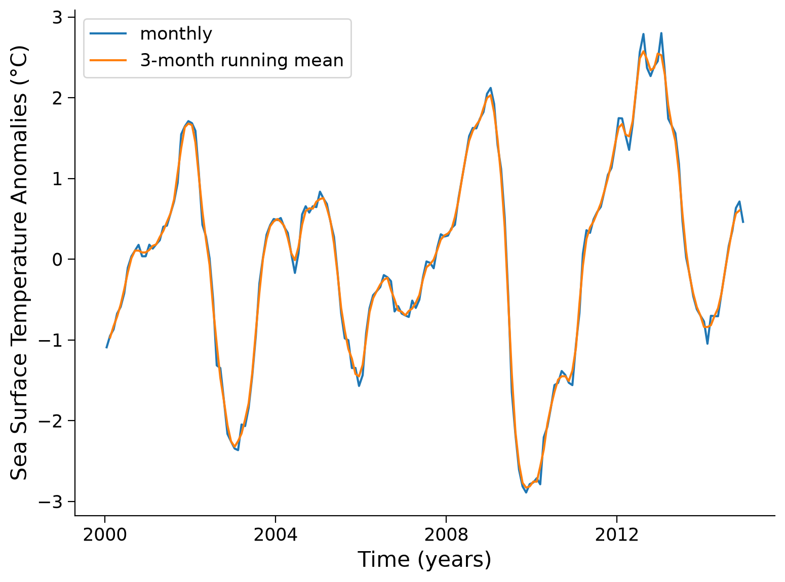
ENSO occurs on interannual timescales (a few years or more). To isolate the variability of this longer-term phenomenon on the Niño 3.4 region, we can smooth out the fluctuations due to variability on shorter timescales. To achieve this, we will apply a 3-month running mean to our time series of SST anomalies.
In other words, even though we have almost the same amount of values in our time series, one SST anomaly entry now also depends on its neighboring months. The neighboring entries now influence the extremity of, e.g., a peak, by reducing its height in correspondence with their difference to this fluctuation. In summary, this removes short-term deviations and highlights when the signal is sustained over a longer time.
# smooth using a centered 3 month running mean
oni_index = tos_nino34_anom_mean.rolling( time = 3, center=True ).mean()
# define the plot size
fig = plt.figure()

# assign axis
ax = plt.axes()

# plot the monhtly data on the assigned axis
tos_nino34_anom_mean.plot(ax=ax)

# plot the smoothed data on the assigned axis
oni_index.plot(ax=ax)

# add legend
ax.legend(["monthly", "3-month running mean"])

# add ylabel
ax.set_ylabel("Sea Surface Temperature Anomalies (°C)")

# add xlabel
ax.set_xlabel("Time (years)")
Text(0.5, 0, 'Time (years)')
Click here for a description of the plot
Time series of the sea surface temperature anomalies before smoothing (blue) and after smoothing via the rolling mean over 3 months (orange). A few peaks exceed the $\pm$0.5 threshold for at least five consecutive months which is operationally used by NOAA to classify El Niño or La Niña. Data is from the CESM Earth system model's historical simulation for the Sixth Phase of the Coupled Intercomparison Project (CMIP6).Section 3: Identify El Niño and La Niña Events#
We will highlight values in excess of \(\pm\)0.5, roughly corresponding to El Niño (warm) and La Niña (cold) events.
fig = plt.figure()

plt.fill_between(  # plot with color in between
    oni_index.time.data,  # x values
    # top boundary - y values above or equal 0.5
    oni_index.where(oni_index >= 0.5).data,
    0.5,            # bottom boundary - 0.5
    color = "red",  # color
    alpha = 0.9,    # transparency value
)
plt.fill_between(
    oni_index.time.data,
    oni_index.where(oni_index <= -0.5).data,
    -0.5,
    color = "blue",
    alpha = 0.9,
)

oni_index.plot(color="black")          # plot the smoothed data
plt.axhline(0, color="black", lw = 0.5)  # add a black line at x=0
plt.axhline(
    0.5, color="black", linewidth = 0.5, linestyle="dotted"
)  # add a black line at x = 0.5
plt.axhline(
    -0.5, color="black", linewidth = 0.5, linestyle="dotted"
)  # add a black line at x = -0.5

# aesthetics
plt.title("Oceanic Niño Index (ONI)")
plt.xlabel('Time (years)')
plt.ylabel("Sea Surface Temperature Anomalies (°C)")
Text(0, 0.5, 'Sea Surface Temperature Anomalies (°C)')
Click here for a description of the plot
Time series of the 3-month averaged sea surface temperature anomalies with highlighted threshold areas, exceeding +0.5 in red and -0.5 in blue, respectively. A few peaks exceed the $\pm$0.5 threshold for at least five consecutive months which is operationally used by NOAA to classify El Niño or La Niña. Data is from the CESM Earth system model's historical simulation for the Sixth Phase of the Coupled Intercomparison Project (CMIP6).Questions 3:#
Now that we’ve normalized the data and highlighted SST anomalies that correspond to El Niño (warm) and La Niña (cold) events, consider the following questions:
How frequently do El Niño and La Niña events occur over the period of time studied here?
When were the strongest El Niño and La Niña events over this time period?
Considering the ocean-atmosphere interactions that cause El Niño and La Niña events, can you hypothesize potential reasons one El Niño or La Niña event may be stronger than others?
Submit your feedback#
Show code cell source
# @title Submit your feedback
content_review(f"{feedback_prefix}_Questions_3")
Summary#
In this tutorial, we have learned to utilize a variety of Xarray tools to examine variations in SST during El Niño and La Niña events. We’ve practiced loading SST data from the CESM2 model, and masking data using the .where() function for focused analysis. We have also computed climatologies and anomalies using the .groupby() function, and learned to compute moving averages using the .rolling() function. Finally, we have calculated, normalized, and plotted the Oceanic Niño Index (ONI), enhancing our understanding of the El Niño Southern Oscillation (ENSO) and its impacts on global climate patterns.
Resources#
Data from this tutorial can be accessed here.