Tutorial 2: A Lot of Weather Makes Climate - Exploring the ERA5 Reanalysis

Tutorial 2: A Lot of Weather Makes Climate - Exploring the ERA5 Reanalysis#

Week 1, Day 2, Ocean-Atmosphere Reanalysis

Content creators: Momme Hell

Content reviewers: Katrina Dobson, Danika Gupta, Maria Gonzalez, Will Gregory, Nahid Hasan, Paul Heubel, Sherry Mi, Beatriz Cosenza Muralles, Jenna Pearson, Chi Zhang, Ohad Zivan

Content editors: Paul Heubel, Jenna Pearson, Chi Zhang, Ohad Zivan

Production editors: Wesley Banfield, Paul Heubel, Jenna Pearson, Konstantine Tsafatinos, Chi Zhang, Ohad Zivan

Our 2024 Sponsors: NFDI4Earth, CMIP

Tutorial Objectives#

Estimated timing of tutorial: 25 mins

In the previous tutorial, we learned about the El Niño Southern Oscillation (ENSO), which is a specific atmosphere-ocean dynamical phenomenon. You will now examine the atmosphere and the ocean systems more generally.

In this tutorial, you will learn to work with reanalysis data. These data combine observations and models of the Earth system and are a critical tool for weather and climate science. You will first access a specific reanalysis dataset: ECMWF’s ERA5. You will then select variables and slices of interest from the preprocessed file, investigating how important climate variables change on medium-length timescales (hours to months) within a certain region.

By the end of this tutorial, you will be able to:

Access reanalysis data of climatically important variables.
Plot interactive maps to explore changes on various time scales.
Compute and compare time series of different variables from reanalysis data.

Setup#

# installations ( uncomment and run this cell ONLY when using google colab or kaggle )

# !pip install xarray==2024.2 scipy cartopy geoviews cdsapi cftime nc-time-axis
# last supported xaray version, see last comment on this thread: https://github.com/pydata/xarray/issues/8909

import cdsapi
import matplotlib.pyplot as plt
import xarray as xr
import numpy as np
import geoviews as gv
import geoviews.feature as gf
import holoviews

import os
import pooch
import tempfile

from cartopy import crs as ccrs

import warnings
#  Suppress warnings issued by Cartopy when downloading data files
warnings.filterwarnings('ignore')

Install and import feedback gadget#

Helper functions#

Figure Settings#

Video 1: ECMWF Reanalysis#

Submit your feedback#

Section 1: What is Reanalysis Data?#

Reanalysis refers to the process of combining historical observations from a variety of sources, such as weather stations, satellite measurements, and ocean buoys, with numerical models to create a comprehensive and consistent record of past weather and climate conditions. Reanalysis data is a useful tool to examine the Earth’s climate system over a wide range of time scales, from seasonal through decadal to century-scale changes.

There are multiple Earth system reanalysis products (e.g. MERRA-2, NCEP-NCAR, JRA-55C, see an extensive list here), and no single product fits all needs. For this tutorial, you will be using a product from the European Centre for Medium-Range Weather Forecasts (ECMWF) called ECMWF Reanalysis v5 (ERA5). This video from the ECMWF provides you with a brief introduction to the ERA5 product.

Section 1.1: Accessing ERA5 Data#

You will access the data through our OSF cloud storage to simplify the downloading process. If you are keen to download the data yourself or are simply interested in exploring other variables, please have a look into the get_ERA5_reanalysis_data.ipynb notebook, where we use the Climate Data Store (CDS) API to get a subset of the huge ECMWF ERA5 Reanalysis data set.

Let’s select a specific year and month to work with, March of 2018:

# load data: 5 variables of ERA5 reanalysis, subregion, hourly, March 2018
fname_ERA5_allvars = "ERA5_5vars_032018_hourly_NE-US.nc"
url_ERA5_allvars = "https://osf.io/7kcwn/download"
ERA5_allvars = xr.open_dataset(pooch_load(url_ERA5_allvars, fname_ERA5_allvars))

Downloading data from 'https://osf.io/7kcwn/download' to file '/tmp/ERA5_5vars_032018_hourly_NE-US.nc'.

---------------------------------------------------------------------------
timeout                                   Traceback (most recent call last)
File /opt/hostedtoolcache/Python/3.9.18/x64/lib/python3.9/site-packages/urllib3/connectionpool.py:468, in HTTPConnectionPool._make_request(self, conn, method, url, timeout, chunked, **httplib_request_kw)
    464         except BaseException as e:
    465             # Remove the TypeError from the exception chain in
    466             # Python 3 (including for exceptions like SystemExit).
    467             # Otherwise it looks like a bug in the code.
--> 468             six.raise_from(e, None)
    469 except (SocketTimeout, BaseSSLError, SocketError) as e:

File <string>:3, in raise_from(value, from_value)

File /opt/hostedtoolcache/Python/3.9.18/x64/lib/python3.9/site-packages/urllib3/connectionpool.py:463, in HTTPConnectionPool._make_request(self, conn, method, url, timeout, chunked, **httplib_request_kw)
    462 try:
--> 463     httplib_response = conn.getresponse()
    464 except BaseException as e:
    465     # Remove the TypeError from the exception chain in
    466     # Python 3 (including for exceptions like SystemExit).
    467     # Otherwise it looks like a bug in the code.

File /opt/hostedtoolcache/Python/3.9.18/x64/lib/python3.9/http/client.py:1377, in HTTPConnection.getresponse(self)
   1376 try:
-> 1377     response.begin()
   1378 except ConnectionError:

File /opt/hostedtoolcache/Python/3.9.18/x64/lib/python3.9/http/client.py:320, in HTTPResponse.begin(self)
    319 while True:
--> 320     version, status, reason = self._read_status()
    321     if status != CONTINUE:

File /opt/hostedtoolcache/Python/3.9.18/x64/lib/python3.9/http/client.py:281, in HTTPResponse._read_status(self)
    280 def _read_status(self):
--> 281     line = str(self.fp.readline(_MAXLINE + 1), "iso-8859-1")
    282     if len(line) > _MAXLINE:

File /opt/hostedtoolcache/Python/3.9.18/x64/lib/python3.9/socket.py:704, in SocketIO.readinto(self, b)
    703 try:
--> 704     return self._sock.recv_into(b)
    705 except timeout:

File /opt/hostedtoolcache/Python/3.9.18/x64/lib/python3.9/ssl.py:1275, in SSLSocket.recv_into(self, buffer, nbytes, flags)
   1272         raise ValueError(
   1273           "non-zero flags not allowed in calls to recv_into() on %s" %
   1274           self.__class__)
-> 1275     return self.read(nbytes, buffer)
   1276 else:

File /opt/hostedtoolcache/Python/3.9.18/x64/lib/python3.9/ssl.py:1133, in SSLSocket.read(self, len, buffer)
   1132 if buffer is not None:
-> 1133     return self._sslobj.read(len, buffer)
   1134 else:

timeout: The read operation timed out

During handling of the above exception, another exception occurred:

ReadTimeoutError                          Traceback (most recent call last)
File /opt/hostedtoolcache/Python/3.9.18/x64/lib/python3.9/site-packages/requests/adapters.py:667, in HTTPAdapter.send(self, request, stream, timeout, verify, cert, proxies)
    666 try:
--> 667     resp = conn.urlopen(
    668         method=request.method,
    669         url=url,
    670         body=request.body,
    671         headers=request.headers,
    672         redirect=False,
    673         assert_same_host=False,
    674         preload_content=False,
    675         decode_content=False,
    676         retries=self.max_retries,
    677         timeout=timeout,
    678         chunked=chunked,
    679     )
    681 except (ProtocolError, OSError) as err:

File /opt/hostedtoolcache/Python/3.9.18/x64/lib/python3.9/site-packages/urllib3/connectionpool.py:802, in HTTPConnectionPool.urlopen(self, method, url, body, headers, retries, redirect, assert_same_host, timeout, pool_timeout, release_conn, chunked, body_pos, **response_kw)
    800     e = ProtocolError("Connection aborted.", e)
--> 802 retries = retries.increment(
    803     method, url, error=e, _pool=self, _stacktrace=sys.exc_info()[2]
    804 )
    805 retries.sleep()

File /opt/hostedtoolcache/Python/3.9.18/x64/lib/python3.9/site-packages/urllib3/util/retry.py:552, in Retry.increment(self, method, url, response, error, _pool, _stacktrace)
    551 if read is False or not self._is_method_retryable(method):
--> 552     raise six.reraise(type(error), error, _stacktrace)
    553 elif read is not None:

File /opt/hostedtoolcache/Python/3.9.18/x64/lib/python3.9/site-packages/urllib3/packages/six.py:770, in reraise(tp, value, tb)
    769         raise value.with_traceback(tb)
--> 770     raise value
    771 finally:

File /opt/hostedtoolcache/Python/3.9.18/x64/lib/python3.9/site-packages/urllib3/connectionpool.py:716, in HTTPConnectionPool.urlopen(self, method, url, body, headers, retries, redirect, assert_same_host, timeout, pool_timeout, release_conn, chunked, body_pos, **response_kw)
    715 # Make the request on the httplib connection object.
--> 716 httplib_response = self._make_request(
    717     conn,
    718     method,
    719     url,
    720     timeout=timeout_obj,
    721     body=body,
    722     headers=headers,
    723     chunked=chunked,
    724 )
    726 # If we're going to release the connection in ``finally:``, then
    727 # the response doesn't need to know about the connection. Otherwise
    728 # it will also try to release it and we'll have a double-release
    729 # mess.

File /opt/hostedtoolcache/Python/3.9.18/x64/lib/python3.9/site-packages/urllib3/connectionpool.py:470, in HTTPConnectionPool._make_request(self, conn, method, url, timeout, chunked, **httplib_request_kw)
    469 except (SocketTimeout, BaseSSLError, SocketError) as e:
--> 470     self._raise_timeout(err=e, url=url, timeout_value=read_timeout)
    471     raise

File /opt/hostedtoolcache/Python/3.9.18/x64/lib/python3.9/site-packages/urllib3/connectionpool.py:358, in HTTPConnectionPool._raise_timeout(self, err, url, timeout_value)
    357 if isinstance(err, SocketTimeout):
--> 358     raise ReadTimeoutError(
    359         self, url, "Read timed out. (read timeout=%s)" % timeout_value
    360     )
    362 # See the above comment about EAGAIN in Python 3. In Python 2 we have
    363 # to specifically catch it and throw the timeout error

ReadTimeoutError: HTTPSConnectionPool(host='osf.io', port=443): Read timed out. (read timeout=30)

During handling of the above exception, another exception occurred:

ReadTimeout                               Traceback (most recent call last)
Cell In[8], line 4
      2 fname_ERA5_allvars = "ERA5_5vars_032018_hourly_NE-US.nc"
      3 url_ERA5_allvars = "https://osf.io/7kcwn/download"
----> 4 ERA5_allvars = xr.open_dataset(pooch_load(url_ERA5_allvars, fname_ERA5_allvars))

Cell In[4], line 10, in pooch_load(filelocation, filename, processor)
      8     file = os.path.join(shared_location, filename)
      9 else:
---> 10     file = pooch.retrieve(
     11         filelocation,
     12         known_hash=None,
     13         fname=os.path.join(user_temp_cache, filename),
     14         processor=processor,
     15     )
     17 return file

File /opt/hostedtoolcache/Python/3.9.18/x64/lib/python3.9/site-packages/pooch/core.py:239, in retrieve(url, known_hash, fname, path, processor, downloader, progressbar)
    236 if downloader is None:
    237     downloader = choose_downloader(url, progressbar=progressbar)
--> 239 stream_download(url, full_path, known_hash, downloader, pooch=None)
    241 if known_hash is None:
    242     get_logger().info(
    243         "SHA256 hash of downloaded file: %s\n"
    244         "Use this value as the 'known_hash' argument of 'pooch.retrieve'"
   (...)
    247         file_hash(str(full_path)),
    248     )

File /opt/hostedtoolcache/Python/3.9.18/x64/lib/python3.9/site-packages/pooch/core.py:807, in stream_download(url, fname, known_hash, downloader, pooch, retry_if_failed)
    803 try:
    804     # Stream the file to a temporary so that we can safely check its
    805     # hash before overwriting the original.
    806     with temporary_file(path=str(fname.parent)) as tmp:
--> 807         downloader(url, tmp, pooch)
    808         hash_matches(tmp, known_hash, strict=True, source=str(fname.name))
    809         shutil.move(tmp, str(fname))

File /opt/hostedtoolcache/Python/3.9.18/x64/lib/python3.9/site-packages/pooch/downloaders.py:220, in HTTPDownloader.__call__(self, url, output_file, pooch, check_only)
    218     # pylint: enable=consider-using-with
    219 try:
--> 220     response = requests.get(url, timeout=timeout, **kwargs)
    221     response.raise_for_status()
    222     content = response.iter_content(chunk_size=self.chunk_size)

File /opt/hostedtoolcache/Python/3.9.18/x64/lib/python3.9/site-packages/requests/api.py:73, in get(url, params, **kwargs)
     62 def get(url, params=None, **kwargs):
     63     r"""Sends a GET request.
     64 
     65     :param url: URL for the new :class:`Request` object.
   (...)
     70     :rtype: requests.Response
     71     """
---> 73     return request("get", url, params=params, **kwargs)

File /opt/hostedtoolcache/Python/3.9.18/x64/lib/python3.9/site-packages/requests/api.py:59, in request(method, url, **kwargs)
     55 # By using the 'with' statement we are sure the session is closed, thus we
     56 # avoid leaving sockets open which can trigger a ResourceWarning in some
     57 # cases, and look like a memory leak in others.
     58 with sessions.Session() as session:
---> 59     return session.request(method=method, url=url, **kwargs)

File /opt/hostedtoolcache/Python/3.9.18/x64/lib/python3.9/site-packages/requests/sessions.py:589, in Session.request(self, method, url, params, data, headers, cookies, files, auth, timeout, allow_redirects, proxies, hooks, stream, verify, cert, json)
    584 send_kwargs = {
    585     "timeout": timeout,
    586     "allow_redirects": allow_redirects,
    587 }
    588 send_kwargs.update(settings)
--> 589 resp = self.send(prep, **send_kwargs)
    591 return resp

File /opt/hostedtoolcache/Python/3.9.18/x64/lib/python3.9/site-packages/requests/sessions.py:703, in Session.send(self, request, **kwargs)
    700 start = preferred_clock()
    702 # Send the request
--> 703 r = adapter.send(request, **kwargs)
    705 # Total elapsed time of the request (approximately)
    706 elapsed = preferred_clock() - start

File /opt/hostedtoolcache/Python/3.9.18/x64/lib/python3.9/site-packages/requests/adapters.py:713, in HTTPAdapter.send(self, request, stream, timeout, verify, cert, proxies)
    711     raise SSLError(e, request=request)
    712 elif isinstance(e, ReadTimeoutError):
--> 713     raise ReadTimeout(e, request=request)
    714 elif isinstance(e, _InvalidHeader):
    715     raise InvalidHeader(e, request=request)

ReadTimeout: HTTPSConnectionPool(host='osf.io', port=443): Read timed out. (read timeout=30)

ERA5_allvars

You just loaded an xarray dataset, as introduced on the first day. This dataset contains 5 variables covering the Northeastern United States along with their respective coordinates. With this dataset, you have access to our best estimates of climate parameters with a temporal resolution of 1 hour and a spatial resolution of 1/4 degree (i.e. grid points near the Equator represent a ~25 km x 25 km region). This is a lot of data, but still just a fraction of the data available through the full ERA5 dataset.

Section 1.2: Selecting Regions of Interest#

The global ERA5 data over the entire time range is so large that even just one variable would be too large to store on your computer. Here we use preprocessed slices of an example region, to load another region (i.e., a spatial subset) of the data, please check out the get_ERA5_reanalysis_data.ipynb notebook. In this first example, you will load air surface temperature at 2 meters data for a small region in the Northeastern United States. In later tutorials, you will have the opportunity to select a region of your choice and explore other climate variables.

The magnitude of the wind vector represents the wind speed

(1)#\[\begin{align} ||u|| = \sqrt{u^2 + v^2} \end{align}\]

which you will use later in the tutorial for time series comparison and discuss in more detail in Tutorial 4. We will calculate that here and add it to our dataset.

# compute ten-meter wind speed, the magnitude of the wind vector
ERA5_allvars["wind_speed"] = np.sqrt(
    ERA5_allvars["u10"] ** 2
    + ERA5_allvars["v10"] ** 2
)
# add name and units to the metadata:
ERA5_allvars["wind_speed"].attrs[
    "long_name"
] = "10-meter wind speed"  # assigning the long name to the attributes
ERA5_allvars["wind_speed"].attrs["units"] = "m/s"  # assigning units
ERA5_allvars

Section 2: Plotting Spatial Maps of Reanalysis Data#

First, let’s plot the region’s surface temperature for the first time step of the reanalysis dataset. To do this let’s extract the 2m air temperature data from the dataset that contains all the variables.

ds_surface_temp_2m = ERA5_allvars.t2m
ds_surface_temp_2m

We will be plotting this a little bit differently than you have previously plotted a map (and differently from how you will plot in most tutorials) so we can look at a few times steps interactively later. To do this we are using the packages geoviews and holoviews.

holoviews.extension("bokeh")

dataset_plot = gv.Dataset(ds_surface_temp_2m.isel(time=0))  # select the first time step

# create the image
images = dataset_plot.to(
    gv.Image, ["longitude", "latitude"], ["t2m"], "hour"
)

# aesthetics, add coastlines etc.
images.opts(
    cmap="coolwarm",
    colorbar=True,
    width=600,
    height=400,
    projection=ccrs.PlateCarree(),
    clabel="2m Air Temperature (K)",
) * gf.coastline

In the above figure, coastlines are shown as black lines. Most of the selected region is land, with some ocean (lower right) and a lake (top middle).

Next, we will examine variability at two different frequencies using interactive plots:

Hourly variability
Daily variability

Note that in the previous tutorial, you computed the monthly variability, or climatology, but here you only have one month of data loaded (March 2018). If you are curious about longer timescales you will visit this in the next tutorial!

# average temperatures over the whole month after grouping by the hour
ds_surface_temp_2m_hour = ds_surface_temp_2m.groupby("time.hour").mean()

# interactive plot of hourly frequency of surface temperature
# this cell may take a little longer as it contains several maps in a single plotting function
dataset_plot = gv.Dataset(
    ds_surface_temp_2m_hour.isel(hour=slice(0, 12))
)  # only the first 12 time steps (midnight to noon), as it is a time-consuming task
images = dataset_plot.to(
    gv.Image, ["longitude", "latitude"], ["t2m"], "hour"
)
images.opts(
    cmap="coolwarm",
    colorbar=True,
    width=600,
    height=400,
    projection=ccrs.PlateCarree(),
    clabel="2m Air Temperature (K)",
) * gf.coastline

# average temperatures over the whole day after grouping by the day
ds_surface_temp_2m_day = ds_surface_temp_2m.groupby("time.day").mean()

# interactive plot of daily frequency of surface temperature
# this cell may take a little longer as it contains several maps in a single plotting function holoviews.extension('bokeh')
dataset_plot = gv.Dataset(
    ds_surface_temp_2m_day.isel(day=slice(0, 10))
)  # only the first 10 time steps, as it is a time-consuming task
images = dataset_plot.to(
    gv.Image, ["longitude", "latitude"], ["t2m"], "day"
)
images.opts(
    cmap="coolwarm",
    colorbar=True,
    width=600,
    height=400,
    projection=ccrs.PlateCarree(),
    clabel="2m Air Temperature (K)",
) * gf.coastline

Questions 2#

What differences do you notice between the hourly and daily interactive plots, and are there any interesting spatial patterns of these temperature changes?

Click for solution

Submit your feedback#

Section 3: Plotting Time Series of Reanalysis Data#

Section 3.1: Surface Air Temperature Time Series#

You have demonstrated that there are a lot of changes in surface temperature within a day and between days. It is crucial to understand this temporal variability in the data when performing climate analysis.

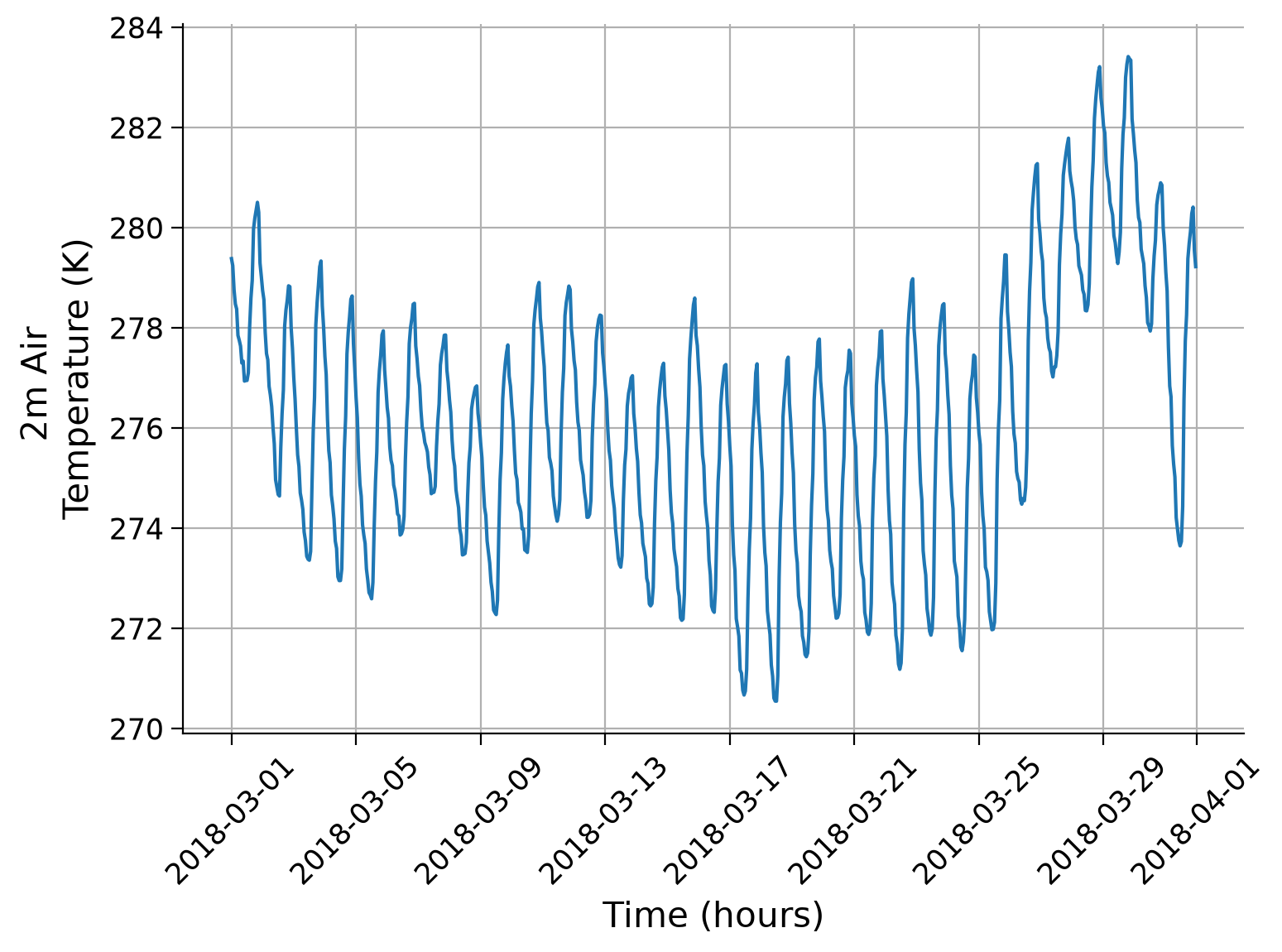
Rather than plotting interactive spatial maps for different timescales, in this last section, you will create a time series of surface air temperature from the data you have already examined to look at variability on longer than daily timescales. Instead of taking the mean in time to create maps, you will now take the mean in space to create time series.

Note that the spatially averaged data will now only have a time coordinate, making it a time series (ts).

# find weights (this is a regular grid so we can use cos(latitude))
weights = np.cos(np.deg2rad(ds_surface_temp_2m.latitude))
weights.name = "weights"
# take the weighted spatial mean since the latitude range of the region of interest is large
ds_surface_temp_2m_ts = ds_surface_temp_2m.weighted(weights).mean(["longitude", "latitude"])
ds_surface_temp_2m_ts

# plot the time series of surface temperature
fig, ax = plt.subplots()

ax.plot(ds_surface_temp_2m_ts.time, ds_surface_temp_2m_ts)

# aesthetics
ax.set_xlabel("Time (hours)")
ax.set_ylabel("2m Air \nTemperature (K)")
ax.xaxis.set_tick_params(rotation=45)
ax.grid(True)

Questions 3.1#

What is the dominant source of the high frequency (short timescale) variability?
What drives the lower frequency variability?
Would the ENSO variablity that you computed in the previous tutorial show up here? Why or why not?

Click for solution

Submit your feedback#

Section 3.2: Comparing Time Series of Multiple Variables#

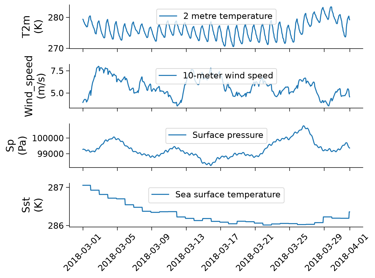
Below you will calculate the time series of the surface air temperature which we just plotted, alongside the time series of several other ERA5 variables for the same period and region: 10-meter wind speed (wind_speed), atmospheric surface pressure (sp), and sea surface temperature (sst).

ERA5_allvars_ts = ERA5_allvars.weighted(weights).mean(["longitude", "latitude"])
ERA5_allvars_ts

plot_vars = [
    "t2m",        # air temperature at 2 meters
    "wind_speed", # magnitude of the wind vector, cf. Section 1
    "sp",         # surface air pressure
    "sst",        # sea surface temperature
]

fig, ax_list = plt.subplots(len(plot_vars), 1, sharex=True)

for var, ax in zip(plot_vars, ax_list):                   # loop through variables and figure axes
    legend_entry = ERA5_allvars[var].attrs["long_name"]                     # create legend entry
    ax.plot(ERA5_allvars_ts.time, ERA5_allvars_ts[var], label=legend_entry) # plot time series

    # aesthetics
    ax.set_ylabel(f'{var.capitalize()}\n({ERA5_allvars[var].attrs["units"]})') # add ylabel w/ units
    ax.xaxis.set_tick_params(rotation=45)                                      # rotate dates of xticks
    ax.legend(loc='upper center')                       # add legend with shared location (upper center)

Questions 3.2#

Which variable shows variability that is dominated by:

The diurnal cycle?
The synoptic [~5 day] scale?
A mix of these two timescales?
Longer timescales?

Click for solution

Submit your feedback#

Summary#

In this tutorial, you learned how to access and process ERA5 reanalysis data. You are now able to select specific slices within the reanalysis dataset and perform operations such as taking spatial and temporal averages to plot them interactively.

You also looked at different climate variables to distinguish and identify the variability present at different timescales.

Resources#

Data for this tutorial can be accessed here. We summarized the download procedure in a separate notebook named get_ERA5_reanalysis_data.ipynb.

Tutorial 2: A Lot of Weather Makes Climate - Exploring the ERA5 Reanalysis

Contents

Tutorial 2: A Lot of Weather Makes Climate - Exploring the ERA5 Reanalysis#

Tutorial Objectives#

Setup#

Install and import feedback gadget#

Helper functions#

Figure Settings#

Video 1: ECMWF Reanalysis#

Submit your feedback#

Section 1: What is Reanalysis Data?#

Section 1.1: Accessing ERA5 Data#

Section 1.2: Selecting Regions of Interest#

Section 2: Plotting Spatial Maps of Reanalysis Data#

Questions 2#

Submit your feedback#

Section 3: Plotting Time Series of Reanalysis Data#

Section 3.1: Surface Air Temperature Time Series#

Questions 3.1#

Submit your feedback#

Section 3.2: Comparing Time Series of Multiple Variables#

Questions 3.2#

Submit your feedback#

Summary#

Resources#